通过 sklearn 进行大规模机器学习

sklearn 是 python 中一个非常著名的机器学习库，但是一般都是在单机上使用而不支持分布式计算，因此往往跟大规模的机器学习扯不上关系。这里通过 sklearn 进行的大规模机器学习指的也不是分布式机器学习，而是指当数据量比内存要大时怎么通过 sklearn 进行机器学习，更准确来说是 out-of-core learning， 这里涉及到的一个核心思想是将数据转化为流式输入，然后通过 SGD 更新模型的参数，当然其中还涉及到一些其他的细节和trick，下面会详细描述。

out-of-core learning

上面的问题也称为 out-of-core learning， 指的是机器的内存无法容纳训练的数据集， 但是硬盘可容纳这些数据，这种情况在数据集较大的时候比较常见，一般有两种解决方法：sampling 与 mini-batch learning。

第一种方法是 sampling（采样），采样 可以针对样本数目或样本特征，能够减少样本的数量或者feature的数目，两者均能减小整个数据集所占内存，但是采样无可避免地会丢失掉原来数据集中的一些信息（当数据没有冗余的时候），这会导致 variance inflation 问题，也就是进行若干次采样，每次训练得出的模型之间差异都比较大。用 bias-variance 来解释就是出现了high variance，原因是每次采样得到的数据中都有随机噪声，而模型拟合了这些没有规律的噪声，从而导致了每次得到的模型都不一样。

解决采样带来的 high-variance 问题，可以通过训练多个采样模型，然后将其进行集成，采用这种思路典型的方法有 bagging。

第二种方法是 mini-batch learning，这种方法不同于 sampling， 利用了全部的数据， 只是每次只用一部分样本（可以是一个样本，也可以是多个样本）来训练模型，通过增加迭代的次数可以近似用全部数据集训练的效果，这种方法需要训练的算法的支持，SGD 恰好就能够提供这种模式的训练，因此 SGD 是这种模式训练的核心。下面也主要针对这种方法进行讲述。

通过 SGD 进行训练时，需要流式（streaming）读取训练样本，同时注意的是要将样本的顺序随机打乱,以消除样本顺序带来的信息，如先用正样本训练，再用负样本训练，模型会偏向于将样本预测为负。下面主要讲述如何将磁盘上的数据流式化并送入到模型中进行训练。

流式读取数据

文件读取

这里读取的数据的格式是每行存储一个样本。最简单的方法就是通过 python 读取文件的 readline 方法实现

with open(source_file, 'rb') as f:
    line = f.readline()
    while line:
        # data processing
        # training
        line = f.readline()

而往往训练文件都是 csv 格式的，此时需要丢弃第一行，同时可通过 csv 模块进行读取，下面以这个数据文件为例说明：https://archive.ics.uci.edu/ml/machine-learning-databases/00275/Bike-Sharing-Dataset.zip

SEP = ',' 
with open(source_file, 'rb') as f:
    iterator = csv.reader(f, delimiter = SEP)
    for n, row in enumerate(iterator):
        if n == 0:
            header = row
        else:
            # data processing
            # training
            pass
    print ('Total rows: %i' % (n+1))
    print ('Header: %s' % ', '.join(header))
    print ('Sample values: %s' % ', '.join(row))

输出为

Total rows: 17380
Header: instant, dteday, season, yr, mnth, hr, holiday, weekday, workingday, weathersit, temp, atemp, hum, windspeed, casual, registered, cnt
Sample values: 17379, 2012-12-31, 1, 1, 12, 23, 0, 1, 1, 1, 0.26, 0.2727, 0.65, 0.1343, 12, 37, 49

在上面的例子中，每个样本是就是一个 row（list 类型），样本的 feature 只能通过 row[index] 方式获取，假如要通过 header 中的名称获取， 可以修改上面获取 iterator 的代码，用 csv.DictReader(f, delimiter = SEP) 来获取 iterator，此时得到的 row 会是一个 dictionary，key 为 header 中的列名，value 为对应的值; 对应的代码为

with open(source_file, 'rb') as R:
    iterator = csv.DictReader(R, delimiter=SEP)
    for n, row in enumerate(iterator):
        # data processing
        # training
        pass
    print ('Total rows: %i' % (n+1))
    print ('Sample values: %s' % row)

输出为

Total rows: 17379
Sample values: {'mnth': '12', 'cnt': '49', 'holiday': '0', 'instant': '17379', 'temp': '0.26', 'dteday': '2012-12-31', 'hr': '23', 'season': '1', 'registered': '37', 'windspeed': '0.1343', 'atemp': '0.2727', 'workingday': '1', 'weathersit': '1', 'weekday': '1', 'hum': '0.65', 'yr': '1', 'casual': '12'}

除了通过 csv 模块进行读取，还可以通过 pandas 模块进行读取，pandas 模块可以说是处理 csv 文件的神器，csv 每次只能读取一条数据，而 pandas 可以指定每次读取的数据的数目，如下所示

import pandas as pd
CHUNK_SIZE = 1000
with open(source_file, 'rb') as R:
    iterator = pd.read_csv(R, chunksize=CHUNK_SIZE) 
    for n, data_chunk in enumerate(iterator):
        print ('Size of uploaded chunk: %i instances, %i features' % (data_chunk.shape))
        # data processing
        # training
        pass
    print ('Sample values: \n%s' % str(data_chunk.iloc[0]))

对应的输出为

Size of uploaded chunk: 1000 instances, 17 features
Size of uploaded chunk: 1000 instances, 17 features
Size of uploaded chunk: 1000 instances, 17 features
Size of uploaded chunk: 1000 instances, 17 features
Size of uploaded chunk: 1000 instances, 17 features
Size of uploaded chunk: 1000 instances, 17 features
Size of uploaded chunk: 1000 instances, 17 features
Size of uploaded chunk: 1000 instances, 17 features
Size of uploaded chunk: 1000 instances, 17 features
Size of uploaded chunk: 1000 instances, 17 features
Size of uploaded chunk: 1000 instances, 17 features
Size of uploaded chunk: 1000 instances, 17 features
Size of uploaded chunk: 1000 instances, 17 features
Size of uploaded chunk: 1000 instances, 17 features
Size of uploaded chunk: 1000 instances, 17 features
Size of uploaded chunk: 1000 instances, 17 features
Size of uploaded chunk: 1000 instances, 17 features
Size of uploaded chunk: 379 instances, 17 features
Sample values: 
instant            17001
dteday        2012-12-16
season                 4
yr                     1
mnth                  12
hr                     3
holiday                0
weekday                0
workingday             0
weathersit             2
temp                0.34
atemp             0.3333
hum                 0.87
windspeed          0.194
casual                 1
registered            37
cnt                   38
Name: 17000, dtype: object

数据库读取

上面的是直接从文件中读取的数据，但是数据也可能存在数据库中，因为通过数据库不经能够有效进行增删查改等操作，而且通过 Database Normalization 能够在不丢失信息的基础上减少数据冗余性。

假设上面的数据已经存储在 SQLite 数据库中，则流式读取的方法如下

import sqlite3
import pandas as pd

DB_NAME = 'bikesharing.sqlite'
CHUNK_SIZE = 2500

conn = sqlite3.connect(DB_NAME)
conn.text_factory = str  # allows utf-8 data to be stored     
sql = "SELECT H.*, D.cnt AS day_cnt FROM hour AS H INNER JOIN day as D ON (H.dteday = D.dteday)"
DB_stream = pd.io.sql.read_sql(sql, conn, chunksize=CHUNK_SIZE)
for j,data_chunk in enumerate(DB_stream):
    print ('Chunk %i -' % (j+1)),
    print ('Size of uploaded chunk: %i istances, %i features' % (data_chunk.shape))
    # data processing
    # training
    pass

输出为

Chunk 1 - Size of uploaded chunk: 2500 istances, 18 features
Chunk 2 - Size of uploaded chunk: 2500 istances, 18 features
Chunk 3 - Size of uploaded chunk: 2500 istances, 18 features
Chunk 4 - Size of uploaded chunk: 2500 istances, 18 features
Chunk 5 - Size of uploaded chunk: 2500 istances, 18 features
Chunk 6 - Size of uploaded chunk: 2500 istances, 18 features
Chunk 7 - Size of uploaded chunk: 2379 istances, 18 features

样本的读取顺序

上面简单提到了通过 SGD 训练模型的时候，需要注意样本的顺序必须要是随机打乱的。

假如给定一批样本，然后用整批的样本来更新，那么就不存在样本的读取顺序问题；但是由于像 SGD 这种 online learning 的训练模式，越是后面才读取的样本，模型一般会拟合得更好，因为这是模型最近看到了这些样本且针对这些样本进行了调整。

这样的特性有其好处，如处理时间序列的数据时，由于对最近时间的数据拟合得更好，因此不会受到时间太久远的数据的影响，但是在更多的情况下，这种由样本顺序带来的是有弊无益的，如上面提到的先用全部的正样本训练，再用全部的负样本训练。因此有必要对数据先进行 shuffle ，然后再通过 SGD 来进行训练。

假如内存能够容纳这些数据， 那么所有的数据可以在内存中进行一次 shuffle；假如无法容纳，则可以将整个大的数据文件分为若干个小的文件，分别进行 shuffle ，然后再拼接起来，拼接时也不按照原来的顺序，而是进行 shuffle 后再拼接， 下面是这两种 shuffle 方法的实现代码。

在内存中进行 shuffle 之前可以通过 zlib 对样本先进行压缩，从而让内存可以容纳更多的样本，实现代码如下

import zlib
from random import shuffle

def ram_shuffle(filename_in, filename_out, header=True):
    with open(filename_in, 'rb') as f:
        zlines = [zlib.compress(line, 9) for line in f]
        if header:
            first_row = zlines.pop(0)
    shuffle(zlines)
    with open(filename_out, 'wb') as f:
        if header:
            f.write(zlib.decompress(first_row))
        for zline in zlines:
            f.write(zlib.decompress(zline))

基于磁盘的 shuffle 方法首先将整个文件划分为若干个小文件，然后再进行 shuffle， 为了能够实现整个数据集更彻底的 shuffle ，可以将上面的过程重复几遍，同时每次都改变划分的文件的大小，实现的代码如下

from random import shuffle
import pandas as pd
import numpy as np
import os

def disk_shuffle(filename_in, filename_out, header=True, iterations = 3, CHUNK_SIZE = 2500, SEP=','):
    for i in range(iterations):
        with open(filename_in, 'rb') as R:
            iterator = pd.read_csv(R, chunksize=CHUNK_SIZE) 
            for n, df in enumerate(iterator):
                if n==0 and header:
                    header_cols =SEP.join(df.columns)+'\n'
                df.iloc[np.random.permutation(len(df))].to_csv(str(n)+'_chunk.csv', index=False, header=False, sep=SEP)
        ordering = list(range(0,n+1))
        shuffle(ordering)
        with open(filename_out, 'wb') as W:
            if header:
                W.write(header_cols)
            for f in ordering:
                with open(str(f)+'_chunk.csv', 'r') as R:
                    for line in R:
                        W.write(line)
                os.remove(str(f)+'_chunk.csv')
        filename_in = filename_out
        CHUNK_SIZE = int(CHUNK_SIZE / 2)

sklearn 中的 SGD

通过前面的步骤可以将数据以流式输入，下面接着就是要通过 SGD 进行训练，在 sklearn 中， sklearn.linear_model.SGDClassifier 和 sklearn.linear_model.SGDRegressor 均是通过 SGD 实现，只是一个用于分类，一个用于回归。下面以 sklearn.linear_model.SGDClassifier 为例进行简单说明，更详细的内容可参考其官方文档。这里仅对其几个参数和方法进行简单的讲解。

需要注意的参数有：

• loss : 表示具体的分类器，可选的值为 hinge、log、modified_huber、squared_hinge、perceptron；如 hinge 表示 SVM 分类器，log 表示logistics regression等
• penalty：正则项，用于防止过拟合(默认为 L2 正则项)
• learning_rate: 表示选择哪种学习速率方案，共有三种：constant、optimal、invscaling，各种详细含义可参考官方文档

需要注意的方法主要就是 partial_fit(X, y, classes), X 和 y 是每次流式输入的数据，而 classes 则是具体的分类数目, 若 classes 数目大于2，则会根据 one-vs-rest 规则训练多个分类器。

需要注意的是 partial_fit 只会对数据遍历一次，需要自己显式指定遍历的次数，如下是使用 sklearn 中的 SGDClassfier 的一个简单例子。

from sklearn import linear_model
import pandas as pd

CHUNK_SIZE = 1000
n_iter = 10  # number of iteration over the whole dataset
n_class = 7

model = linear_model.SGDClassifier(loss = 'hinge', penalty ='l1',)
for _ in range(n_iter): 
    with open(source_file, 'rb') as R:
        iterator = pd.read_csv(R, chunksize=CHUNK_SIZE) 
        for n, data_chunk in enumerate(iterator):
            model.partial_fit(data_chunk.x, data_chunk.y, classes = np.array(range(0, n_class)))

流式数据中的特征工程

feature scaling

对于 SGD 算法，特征的 scaling 会影响其优化过程，也就是只有将特征标准化（均值为0，方差为1）或归一化（处于 [0,1] 内）才能加快算法收敛的速度，但是由于数据不能一次读入内存，如果需要标准化或归一化，需要对数据遍历 2 次，第一次遍历是为了求特征的均值和方差（标准化需要）或最大最小值（归一化需要），第二次遍历便可以用上面的均值、方差、最大值，最小值等值进行标准化。

由于数据是流式输入的，求解均值、最大值、最小值都没有什么问题，但是求解方差的公式为( \(\mu\) 为均值）

\[\sigma^2 = \frac{1}{n} \sum_x(x-\mu)^2\]

只有知道均值才能求解， 这意味着只有遍历一次求得 \(\mu\) 后才能求 \(\sigma^2\), 这无疑会增加求解的时间，下面对这个公式进行简单的变换，使得 \(\mu\) 和 \(\sigma^2\) 能够同时求出

假如当前有 \(n\) 个样本，当前的均值 \(\mu'\) 可以简单求出，而当前的方差 \(\sigma'^2\) 可通以下公式求解

\[\sigma'^2 = \frac{1}{n} \sum_x(x^2 - 2x\mu' + \mu'^2) = \frac{1}{n} \sum_x(x^2) - \frac{1}{n}(2n\mu'^2 - n\mu'^2) = \frac{1}{n} \sum_x(x^2) - \mu'^2\]

通过这个公式，可以遍历一次便求出任意个样本的方差，下面通过这个公式求解均值和方差随着样本数量变化而变化的情况，并比较进行 shuffle 前后两者在均值和方差上的区别。

# calculate the running mean,standard deviation, and range reporting the final result
import os, csv
raw_source = 'bikesharing/hour.csv' # unshuffle
shuffle_source = 'bikesharing/shuffled_hour.csv'

def running_statistic(source):
    SEP=','
    running_mean = list()
    running_std = list()
    with open(local_path+'/'+source, 'rb') as R:
        iterator = csv.DictReader(R, delimiter=SEP)
        x = 0.0
        x_squared = 0.0
        for n, row in enumerate(iterator):
            temp = float(row['temp'])
            if n == 0:
                max_x, min_x = temp, temp
            else:
                max_x, min_x = max(temp, max_x),min(temp, min_x)
            x += temp
            x_squared += temp**2
            running_mean.append(x / (n+1))
            running_std.append(((x_squared - (x**2)/(n+1))/(n+1))**0.5)
            # DATA PROCESSING placeholder
            # MACHINE LEARNING placeholder
            pass
        print ('Total rows: %i' % (n+1))
        print ('Feature \'temp\': mean=%0.3f, max=%0.3f, min=%0.3f,sd=%0.3f' \
               % (running_mean[-1], max_x, min_x, running_std[-1]))
        return running_mean, running_std
print '===========raw data file==========='
raw_running_mean, raw_running_std = running_statistic(raw_source)
print '===========shuffle data file==========='
shuffle_running_mean, shuffle_running_std = running_statistic(shuffle_source)

输出如下

===========raw data file===========
Total rows: 17379
Feature 'temp': mean=0.497, max=1.000, min=0.020,sd=0.193
===========shuffle data file===========
Total rows: 17379
Feature 'temp': mean=0.497, max=1.000, min=0.020,sd=0.193

两者的统计数据一致，符合要求，下面再看看两者的均值和方差随着时间如何变化，也就是将上面得到的 running_mean 和 running_std 进行可视化

# plot how such stats changed as data was streamed from disk
# get an idea about how many instances are required before getting a stable mean and standard deviation estimate
import matplotlib.pyplot as plt
%matplotlib inline
for mean, std in ((raw_running_mean, raw_running_std), (shuffle_running_mean, shuffle_running_std)):
    plt.plot(mean,'r-', label='mean')
    plt.plot(std,'b-', label='standard deviation')
    plt.ylim(0.0,0.6)
    plt.xlabel('Number of training examples')
    plt.ylabel('Value') 
    plt.legend(loc='lower right', numpoints= 1)
    plt.show()
# The difference in the two charts reminds us of the importance of randomizing the order of the observations. 

得到的结果如下

原始的文件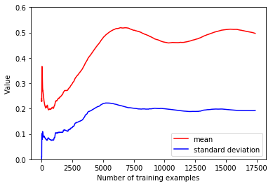

shuffle 后的文件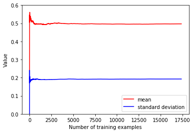

可以看到，经过 shuffle 后的数据的均值和方差很快就达到了稳定的状态，可以让 SGD 算法更快地收敛，这也从另一个角度验证了 shuffle 的必要性。

hasing trick

对于 categorial feature， 往往要对其进行 one-hot 编码，但是进行 one-hot 编码需要知道这个 feature 所有可能的取值的数量，对于流式输入的数据，可以先遍历一遍数据得到 categorial feature 所有可能取值的数目。除此之外，还可以利用接下来要讲的 hashing trick 对categorical feature 进行 one-hot 编码，这种方法对只能遍历一遍的数据有效。

hahsing trick 利用了 hash 函数，通过hash后取模，将样本的值映射到预先定义好的固定长度的槽列中的某个槽中，这种方法需要对 categorical feature 的所有可能取值有大概的估计，而且可能会出现冲突的情况，但是如果对categorical feature 的所有可能取值有较准确的估计时，冲突的概率会比较低。下面是利用 sklearn 中的 HashingVectorizer 进行这种编码的一个例子

from sklearn.feature_extraction.text import HashingVectorizer
h = HashingVectorizer(n_features=1000, binary=True, norm=None)
sparse_vector = h.transform(['A simple toy example will make clear how it works.'])
print(sparse_vector)

输出如下

(0, 61)	1.0
(0, 271)	1.0
(0, 287)	1.0
(0, 452)	1.0
(0, 462)	1.0
(0, 539)	1.0
(0, 605)	1.0
(0, 726)	1.0
(0, 918)	1.0

这里定义的槽列的长度为1000，即假设字典中的单词数目为 1000， 然后将文本映射到这个槽列中，1 表示有这个单词，0表示没有。

总结

本文主要介绍了如何进行 out-of-core learning，主要思想就是将数据以流式方式读入，然后通过 SGD 算法进行更新，在读入数据之前，首先需要对数据进行 shuffle 操作，消除数据本来的顺序信息等，同时可以让样本的特征的方差和均值更快达到稳定状态。