Four Realms of Large-Scale Machine Learning Frameworks

This article is a repost, the original link can be found here, authored by carbon zhang. This article mainly introduces several key concepts and classic papers in distributed machine learning, including data parallelism and model parallelism, schools of distributed frameworks, parameter servers, and the evolution of synchronization protocols. It is well worth reading.

Background

Since Google published the famous GFS, MapReduce, and BigTable papers, the Internet has officially entered the big data era. The most significant characteristic of big data is its sheer volume - it’s big in every dimension. This article systematically addresses architectural issues encountered when using machine learning to process large-volume data.

With GFS, we have the ability to accumulate massive amounts of data samples, such as online advertising impression and click data, which naturally have positive and negative sample characteristics. Accumulating data for just one or two months can easily yield tens of billions or even hundreds of billions of training samples. How to store such massive samples? What models can learn useful patterns from massive samples? These questions are not only engineering problems but also worth thinking deeply about for every algorithm engineer.

Simple Models or Complex Models

Before the concept of deep learning was proposed, algorithm engineers had very few tools at their disposal - just a handful of relatively fixed models and algorithms like LR, SVM, and perceptron. At that time, to solve an actual problem, algorithm engineers mostly worked on feature engineering. Feature engineering itself didn’t have a very systematic guiding theory (at least no books systematically introducing feature engineering have been seen), so feature construction techniques often appeared bizarre, and whether they worked depended on the problem itself, data samples, model, and luck.

When feature engineering was the main work content for algorithm engineers, attempts to construct new features often largely didn’t work in practice. As far as I know, several major companies’ success rate in feature construction in later stages generally didn’t exceed 20%. In other words, 80% of newly constructed features often had no positive improvement effect. If we give this approach a name, it would be roughly simple model + complex features. Simple models mean algorithms like LR and SVM themselves are not complex, with parameters and expressive power basically showing a linear relationship, easy to understand. Complex features refer to constantly attempting various tricks in feature engineering to construct possibly useful or useless features. The construction of these features might involve various tricks, such as window sliding, discretization, normalization, square root, squaring, Cartesian product, multiple Cartesian products, etc.. By the way, since feature engineering itself doesn’t have particularly systematic theory and summary, beginners who want to construct features need to read more papers, especially papers with similar business scenarios to their own, to learn the author’s methods of analyzing and understanding data and corresponding feature construction techniques from them. Over time, one may form their own knowledge system.

After the concept of deep learning was proposed, people discovered that deep neural networks could perform a certain degree of representation learning. For example, in the image domain, the method of extracting image features through CNN and then classifying them broke the previous algorithm’s ceiling, and by a huge margin. This brought new ideas to all algorithm engineers - since deep learning itself has the ability to extract features, why bother painfully doing manual feature design?

Although deep learning alleviates the pressure of feature engineering to some extent, two points need to be emphasized here:

1. Alleviation doesn’t mean complete solution. Except for specific domains like images, deep learning hasn’t completely achieved absolute advantage in personalized recommendation and other domains. The reason might be that the data’s intrinsic structure in other domains hasn’t yet found the perfect combination like image + CNN.
2. While deep learning alleviates feature engineering, it also brings problems of complex models and lack of interpretability. Algorithm engineers also need to put a lot of thought into network structure design to improve results. In summary, the simple features + complex model represented by deep learning is another way to solve practical problems.

It’s hard to say which of the two modes is better. Taking click-through rate prediction as an example, in computational advertising, massive features + LR is mainstream. According to VC dimension theory, LR’s expressive power is proportional to the number of features, so massive features can completely give LR enough descriptive power. In personalized recommendation, deep learning is just emerging. Currently, Google Play adopted the WDL structure[1], and YouTube adopted the dual DNN structure[2].

Regardless of the mode, when the model becomes large enough, situations arise where model parameters cannot be stored on a single machine. For example, LR weights for tens of billions of features can be dozens of gigabytes, which is difficult to store on many single machines. Large-scale neural networks are even more complex - not only difficult to store on a single machine, but also have strong logical dependencies between parameters. Training super-large-scale models inevitably requires distributed system techniques. This article mainly systematically summarizes some ideas in this regard.

Data Parallelism vs Model Parallelism

Data parallelism and model parallelism are fundamental concepts for understanding large-scale machine learning frameworks. Their origins haven’t been deeply investigated, but they were first seen in Jeff Dean’s blog. Years later, when I started investigating this problem again, I remembered the elder’s lesson: young people are still too naive. If you, like me, once ignored this concept, let’s review it today.

Mu Shuai once gave a very intuitive and classic explanation for these two concepts in this question, but unfortunately, when I wanted to cite it, I found it had been deleted. Let me briefly introduce this analogy: if you want to build two buildings with one construction team, how would you do it? The first approach is to divide people into two groups, each building a building, then decorate after completion. The second approach is one group builds the building, and after the first building is done, the other group decorates the first one, then the first group continues building the second building, then waits for the decoration team to decorate the second building. At first glance, the second method seems to have low parallelism, but the first approach requires every construction worker to have both “building” and “decorating” capabilities, while the second only requires each person to have one of these capabilities. The first approach is similar to data parallelism, while the second reveals the essence of model parallelism.

Data parallelism is relatively easy to understand. When there are many samples, to use all samples to train the model, we can distribute data to different machines, and then each machine iterates on model parameters, as shown in the figure below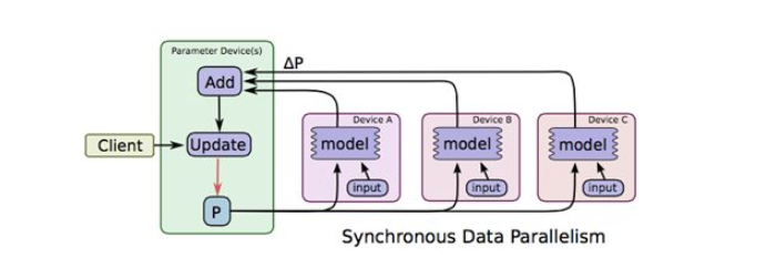

The image is taken from TensorFlow’s paper[3]. In the figure, ABC represents three different machines storing different samples. Model P calculates corresponding increments on each machine, then aggregates and updates on the machine storing parameters. This is data parallelism. Let’s ignore synchronous for now - that’s a concept related to synchronization mechanisms, which will be introduced specifically in the third section.

The concept of data parallelism is simple and doesn’t depend on the specific model, so data parallelism mechanism can serve as a basic feature of the framework, effective for all algorithms. In contrast, model parallelism, due to dependencies between parameters (actually, data parallelism parameter updates may also depend on all parameters, but the difference is that data parallelism often depends on the full parameters from the previous iteration, while model parallelism often has strong dependencies between parameters within the same iteration, such as the sequential dependencies between parameters of different layers in a DNN network formed by the BP algorithm), cannot directly shard model parameters like data parallelism without breaking dependencies. Therefore, model parallelism not only needs to shard the model but also requires a scheduler to control dependencies between parameters. Each model’s dependencies are often different, so model parallelism’s scheduler varies by model and is difficult to make completely universal. CMU’s Eric Xing introduced this here, interested readers can refer to it.

The problem definition of model parallelism can be found in Jeff Dean’s[4], this paper is also a summary related to TensorFlow’s predecessor. The figure in it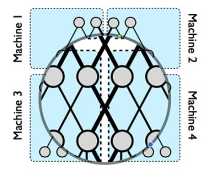

explains the physical picture of model parallelism. When a super-large neural network cannot be stored on one machine, we can cut the network to store on different machines, but to maintain dependencies between different parameter shards, as shown by the thick black lines in the figure, concurrent control is needed between different machines. Dependencies within the same machine, shown by thin black lines, can be controlled within the machine.

How to effectively control the black line parts? As shown in the figure below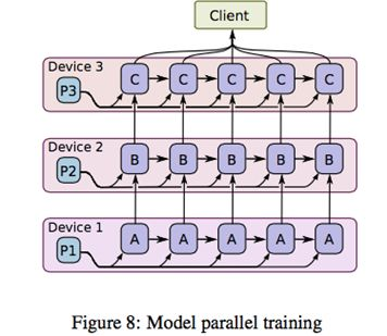

After sharding the model to different machines, we flow parameters and samples together between different machines. ABC in the figure represents different parts of model parameters. Suppose C depends on B, B depends on A. After machine 1 gets one iteration of A, it passes A and necessary sample information to machine 2. Machine 2 updates P2 based on A and samples, and so on. When machine 2 calculates B, machine 1 can start calculating A’s second iteration. Students familiar with CPU pipelining must feel familiar - yes, model parallelism achieves parallelism through data pipelines. Think of the second building construction approach, and you’ll understand the essence of model parallelism.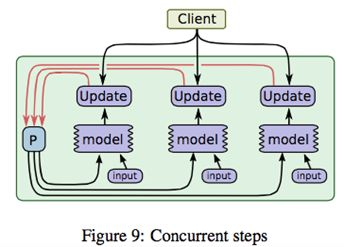

The above figure is a schematic of the scheduler controlling model parameter dependencies. In actual frameworks, DAG (Directed Acyclic Graph) scheduling technology is generally used to implement similar functionality. I haven’t researched this deeply, so I’ll supplement later if there’s opportunity.

Understanding data parallelism and model parallelism is crucial for understanding parameter servers later, but let me first briefly introduce some background information on parallel computing frameworks.

Evolution of Parallel Algorithms

MapReduce Route

Inspired by functional programming, Google published the MapReduce[5] distributed computing method. By cutting tasks into multiple stacked Map+Reduce tasks, complex computing tasks can be completed. The schematic is as follows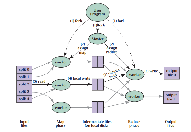

MapReduce has two main problems: first, the primitive semantics are too low-level, requiring significant development effort to write complex algorithms directly; second, it relies on disk for data transfer, and performance can’t keep up with business needs.

To solve MapReduce’s two problems, Matei proposed a new data structure RDD in [6] and built the Spark framework. Spark framework encapsulated a DAG scheduler above MR semantics, greatly lowering the barrier to algorithm usage. For a long time, Spark was almost the representative of large-scale machine learning until Mu Shuai’s parameter server further expanded the field of large-scale machine learning, only then did Spark reveal some shortcomings. As shown below

From the figure, we can see that Spark framework has Driver as the core, with task scheduling and parameter aggregation both at the driver, and driver is a single-machine structure, so Spark’s bottleneck is very obvious - right at the Driver. When the model scale is too large to fit on one machine, Spark cannot run normally. So from today’s perspective, Spark can only be called a medium-scale machine learning framework. Spoiler alert: the company’s open-sourced Angel expanded Spark to a higher level by modifying Driver’s underlying protocol. This will be introduced in more detail later.

MapReduce is not only a framework but also a way of thinking. Google’s pioneering work found a feasible direction for big data analysis. Even today, it’s not outdated. It’s just gradually sinking from the business layer to the framework lower layer where the underlying semantics should be.

MPI Technology

Mu Shuai briefly introduced MPI’s prospects in this question. Unlike Spark, MPI is a system communication API similar to socket, but with support for message broadcasting and other features. Since I haven’t researched MPI deeply, I’ll briefly introduce the advantages and disadvantages. Advantages include system-level support with excellent performance. Disadvantages are also numerous: first, like MR, the primitives are too low-level, so writing algorithms with MPI often requires significant code. Second, MPI-based clusters, if a task fails, often need to restart the entire cluster, and MPI cluster task success rates are not high. Alibaba gave the following figure in [7]: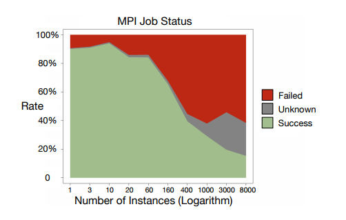

From the figure, we can see MPI job failure rate approaches 50%. MPI isn’t completely without merits. As Mu Shuai said, there are still scenarios on supercomputing clusters. For the industry relying on cloud computing and commodity computers, the cost-effectiveness isn’t high enough. Of course, using MPI for individual worker groups under the parameter server framework might be a good attempt - the KunPeng system in [7] is designed exactly this way.

Parameter Server

Historical Evolution

Mu Shuai divided the history of parameter servers into three phases in [8]. The first generation parameter server emerged from Mu Shuai’s advisor Smola’s [9], as shown below: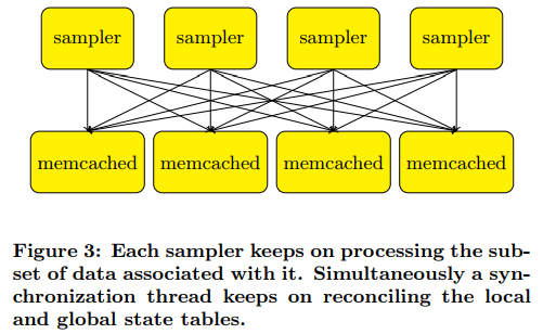

This work only introduced memcached to store key-value data, with different processing threads processing it in parallel. [10] also had similar ideas. The second generation parameter server is called application-specific parameter server, mainly developed for specific applications. The most typical representative should be TensorFlow’s predecessor 4.

The third generation parameter server, also known as the general parameter server framework, was formally proposed by Baidu’s Li Mu. Unlike the first two generations, the third generation parameter server was designed from the start as a general large-scale machine learning framework. To break free from specific applications and algorithms, and create a general large-scale machine learning framework, we must first define the framework’s functions. A framework is about elegantly encapsulating a large amount of repetitive, 琐碎, do-it-once-and-never-again dirty and tedious work, so framework users can focus only on their core logic. What functions does the third generation parameter server encapsulate? Mu Shuai summarized these points, which I’ll reproduce here:

1. Efficient network communication: Since both models and samples are very large, efficient network communication support and high-spec network equipment are indispensable for large-scale machine learning systems.

2. Flexible consistency model: Different consistency models are actually trading off between model convergence speed and cluster computation. Understanding this concept requires some analysis of model performance evaluation, which we’ll leave for the next section.

3. Elastic scalability: Obviously necessary.

4. Fault tolerance: Stragglers or machine failures are very common when large-scale clusters collaborate on computing tasks, so the system design itself must consider how to handle them. Even without failures, machine configurations may need to change at any time due to task timeliness requirements. This also requires the framework to support machine hot-plugging without affecting tasks.

5. Ease of use: Mainly for engineers using the framework for algorithm tuning. Obviously, a difficult-to-use framework has no vitality.

Before formally introducing the third generation parameter server’s main technologies, let’s look at the evolution of large-scale machine learning frameworks from another angle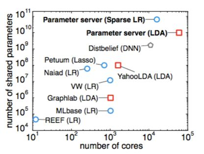

From this figure, we can see that before parameter servers emerged, people had tried various parallel approaches, but often only for specific algorithms or domains, like YahooLDA for LDA algorithm. When model parameters exceeded ten billion, parameter server dominated, with no rivals.

First, let’s look at the basic architecture of the third generation parameter server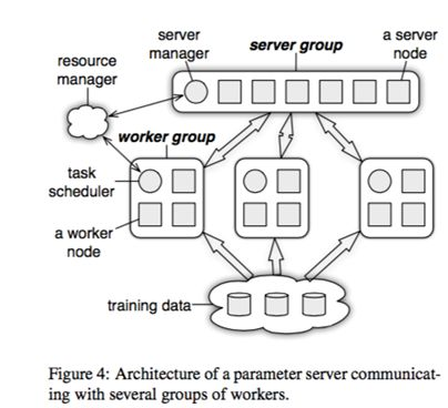

The resource manager in the figure can be set aside for now, because in actual systems this part often reuses existing resource management systems like yarn, mesos, or k8s. The training data at the bottom undoubtedly needs support from distributed file systems like GFS. The rest is the parameter server’s core components.

The figure shows one server group and three worker groups. In actual applications, it’s often similar - one server group, and worker groups configured as needed. The server manager is the management node in the server group, generally without much logic, only making adjustments to maintain consistent hashing when server nodes join or exit.

The task scheduler in the worker group is a simple task coordinator. When a specific task runs, the task scheduler notifies each worker to load its corresponding data, then pulls a parameter shard to update from the server node, calculates the corresponding change for that parameter shard using local data samples, then syncs to the server node. After the server node receives updates from all workers for its parameter shard, it performs one update on the parameter shard.

One issue here is that when different workers run in parallel, they may have different progress due to network, machine configuration, and other external reasons. How to control the workers’ synchronization mechanism is an important topic. See the next section for details.

Synchronization Protocol

This section assumes readers are already familiar with stochastic gradient optimization algorithms. If not, please refer to Andrew Ng’s classic machine learning course’s introduction to SGD, or the book “Introduction to Optimization” that I’ve recommended multiple times.

Let’s first look at the running process of a single-machine algorithm. Assume a model’s parameters are split into three shards k1, k2, k3. For example, you can assume it’s a logistic regression algorithm’s weight vector split into three segments. We also split the training sample set into three shards s1, s2, s3. In a single-machine run, we assume the running sequence is (k1, s1), (k2, s1), (k3, s1), (k1, s2), (k2, s2), (k3, s2)…. Do you understand? We assume using samples in s1 to train parameter shards k1, k2, k3 in turn, then switch to s2. This is the typical single-machine running situation, and we know such a running sequence will eventually converge.

Now let’s parallelize. Assume k1, k2, k3 are distributed on three server nodes, and s1, s2, s3 are distributed on three workers. If we want to maintain the previous computation order, what would happen? When worker1 computes, worker2 and worker3 can only wait. Similarly, when worker2 computes, worker1 and worker3 must wait, and so on. We can see this parallelization doesn’t improve performance, but it does solve the storage problem for super-large-scale models.

To solve the performance problem, the industry started exploring consistency models. The first version was the ASP (Asynchronous Parallel) mode mentioned earlier in 9, where workers completely ignore order - each worker goes at their own pace, finishes an iteration and updates, then continues. This is the freestyle in large-scale machine learning, as shown in the figure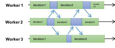

ASP’s advantage is maximizing the cluster’s computing power - all worker machines don’t need to wait. But the disadvantage is also obvious: except for a few models like LDA, ASP protocol may cause the model to fail to converge. That is, SGD completely flies off, and the gradient goes who knows where.

After ASP, another relatively extreme synchronization protocol BSP was proposed. Spark uses this method, as shown in the figure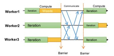

Each worker must run in the same iteration. Only after all workers complete one iteration task does synchronization and shard update between workers and servers occur. This algorithm is very similar to the strictly consistent algorithm, differing only in that the single-machine version’s batch size becomes the total batch size summed from all workers’ individual batch sizes in BSP. Without a doubt, BSP mode is completely identical to single-machine serial in model convergence, differing only in batch size. Meanwhile, since each worker can compute in parallel within one cycle, there’s some parallel capability.

Spark based on this protocol became the de facto hegemony in the machine learning domain for a long time, not without reason. The flaw of this protocol is that the entire worker group’s performance is determined by the slowest worker, called the straggler. Students who’ve read the GFS paper should know stragglers are a very common phenomenon.

Can we compromise between ASP and BSP? The answer is yes - this is what I consider the best synchronization protocol SSP. SSP’s idea is actually very simple: since ASP allows arbitrarily large iteration intervals between different workers, and BSP only allows zero, can we set a constant s? As shown in the figure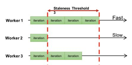

Different workers are allowed to have iteration intervals, but this interval cannot exceed a specified value s. In the figure, s=3.

For detailed introduction to SSP protocol, see [11], where CMU’s Eric Xing details SSP’s definition and its convergence guarantees. Theoretical derivation proves that when constant s is not infinity, the algorithm will definitely enter a converged state after several iterations. Actually, before Eric proposed the theoretical proof, the industry had already tried this approach.

By the way, when evaluating distributed algorithm performance, we generally look at statistical performance and hardware performance separately. The former refers to how many iterations different synchronization protocols require for algorithm convergence, and the latter is the time consumed per iteration. Their relationship is similar to precision and recall, so I won’t elaborate. With SSP, BSP can be obtained by setting s=0, and ASP can be achieved by setting s=infinity.

Core Technologies

Besides parameter server architecture and synchronization protocols, this section briefly introduces other techniques. For detailed understanding, please read Mu Shuai’s doctoral thesis and related published papers directly.

Hot backup and cold backup techniques: To prevent server node crashes from interrupting tasks, two techniques can be used. One is hot backup of parameter shards - each shard is stored on three different server nodes in master-slave form. If the master crashes, the task can quickly restart from the slave.

Besides hot backup, you can also periodically write checkpoint files to distributed file systems to backup parameter shards and their states, further ensuring their safety.

Server node management: Consistent hashing can be used to handle server node joining and exiting, as shown in the figure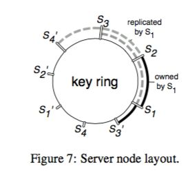

When a server node joins or exits, the server manager is responsible for re-sharding or merging parameters. Note that when managing parameter shards, one shard only needs one lock, which greatly improves system performance and is a key point for parameter servers to be practical.

Four Realms of Large-Scale Machine Learning

Now we can return to our title. What are the four realms of large-scale machine learning?

The division of these four realms is a personal summary from reading, not an industry standard, for reference only.

Realm 1: Parameters can be stored and updated on a single machine

This realm is relatively simple, but parameter servers can still be used to accelerate model training through data parallelism.

Realm 2: Parameters cannot be stored on a single machine, but can be updated on a single machine

This case corresponds to some simple models, like sparse logistic regression. When the number of features exceeds tens of billions, LR’s weight parameters are unlikely to be completely stored on one machine. At this point, parameter server architecture must be used to shard model parameters. But note: SGD’s update formula can be calculated separately for each dimension, but each dimension still needs to use all parameters from the previous iteration (i.e., calculate predicted value f(w)). We shard parameters precisely because we can’t store all parameters on one machine, but now a single worker needs all parameters to calculate the gradient for a parameter shard - isn’t this contradictory? Is it possible?

The answer is yes, because individual samples’ features have very high sparsity. For example, in a model with tens of billions of features, a single training sample often has non-zero values for only a very small portion of features, with all others being 0 (assuming features have been discretized).

Therefore, when calculating f(w), you only need to pull the weights for features that are non-zero. Some articles estimate that at this level of systems, sparsity is often below 0.1% (or 0.01%, not very precise, roughly this). Such sparsity allows single machines to calculate f(w) without any hindrance.

Currently, the company’s open-sourced Angel and the system AILab is working on are at this realm. Native Spark hasn’t reached this realm and can only hang around in the small-to-medium scale circle. Angel’s modified Spark based on Angel has reached this realm.

Realm 3: Parameters cannot be stored or updated on a single machine, but model parallelism is not needed

Realm 3 follows Realm 2. When there are tens of billions of features and the features are relatively dense, the computing framework needs to enter this realm. At this point, a single worker has limited capability and cannot fully load a sample, nor can it fully calculate f(w). What to do? Actually, it’s very simple - anyone who’s studied linear algebra knows matrices can be partitioned. Vectors are the simplest matrices, so naturally they can be calculated in segments. The scheduler just needs to support operator partitioning.

Realm 4: Parameters cannot be stored or updated on a single machine, and model parallelism is needed

Computing frameworks entering this level can be considered world-class. They can handle super-large-scale neural networks. This is also the most typical application scenario. At this point, not only can model parameters not be stored on a single machine, but within the same iteration, there are strong dependencies between model parameters. See Jeff Dean’s introduction to DistBelief for model sharding.

At this point, a coordinator component needs to be added for model parallelism’s concurrent control. At the same time, the parameter server framework needs to support namespace sharding. The coordinator represents dependencies through namespaces.

Dependencies between parameters vary by model, so it’s difficult to abstract a general coordinator. Instead, a DAG graph of the entire computing task must be generated through a script parser in some form, then completed through a DAG scheduler. For an introduction to this problem, refer to Eric Xing’s sharing.

TensorFlow

Currently, well-known deep learning frameworks in the industry include Caffe, MXNet, Torch, Keras, Theano, etc., but the hottest one should be Google’s TensorFlow. Let me break it down briefly.

Quite a few figures earlier are cited from this paper. From TF’s paper, the TF framework itself supports both model parallelism and data parallelism, with a built-in parameter server module. But from the exposed APIs in the open-source version, TF cannot be used for sparse LR models with 10B-level features. The reason is that the exposed APIs only support parameter sharding between different layers of the neural network, while super-large-scale LR can be viewed as a single neural unit - TF doesn’t support sharding a single neural unit’s parameters onto multiple parameter server nodes.

Of course, with Google’s capability, they can absolutely achieve the fourth realm. The reason for not exposing it might be based on other commercial considerations, like promoting their cloud computing services.

In summary, personally, if the fourth realm can be achieved, it can currently be considered a world-class large-scale machine learning framework. From Mu Shuai’s slides alone, he once achieved this. Google internally should have no problem either. The third realm should be domestic first-class, and the second realm should be domestic forefront.

Other

Resource Management

The part not covered in this article is resource management. Large-scale machine learning framework deployed clusters often consume significant resources and need dedicated resource management tools to maintain. Yarn and Mesos are both leaders in this area, so I won’t introduce the details.

Equipment

Besides resource management tools, deploying large-scale machine learning clusters itself has some hardware requirements. Although theoretically, all commodity machines can be used to build such clusters, considering performance, we recommend using high-memory machines with 10GbE or faster network cards. Without ultra-fast network cards, parameter transfer and sample loading would be quite painful.

References

[1] Cheng H T, Koc L, Harmsen J, et al. Wide & deep learning for recommender systems[C]//Proceedings of the 1st Workshop on Deep Learning for Recommender Systems. ACM, 2016: 7-10.

[2] Covington P, Adams J, Sargin E. Deep neural networks for youtube recommendations[C]//Proceedings of the 10th ACM Conference on Recommender Systems. ACM, 2016: 191-198.

[3] Abadi M, Agarwal A, Barham P, et al. Tensorflow: Large-scale machine learning on heterogeneous distributed systems[J]. arXiv preprint arXiv:1603.04467, 2016.

[4] Dean J, Corrado G, Monga R, et al. Large scale distributed deep networks[C]//Advances in neural information processing systems. 2012: 1223-1231.

[5] Dean J, Ghemawat S. MapReduce: simplified data processing on large clusters[J]. Communications of the ACM, 2008, 51(1): 107-113.

[6] Zaharia M, Chowdhury M, Das T, et al. Resilient distributed datasets: A fault-tolerant abstraction for in-memory cluster computing[C]//Proceedings of the 9th USENIX conference on Networked Systems Design and Implementation. USENIX Association, 2012: 2-2.

[7] Zhou J, Li X, Zhao P, et al. KunPeng: Parameter Server based Distributed Learning Systems and Its Applications in Alibaba and Ant Financial[C]//Proceedings of the 23rd ACM SIGKDD International Conference on Knowledge Discovery and Data Mining. ACM, 2017: 1693-1702.

[8] Li M, Andersen D G, Park J W, et al. Scaling Distributed Machine Learning with the Parameter Server[C]//OSDI. 2014, 14: 583-598.

[9] Smola A, Narayanamurthy S. An architecture for parallel topic models[J]. Proceedings of the VLDB Endowment, 2010, 3(1-2): 703-710.

[10] Power R, Li J. Piccolo: Building Fast, Distributed Programs with Partitioned Tables[C]//OSDI. 2010, 10: 1-14.

[11] Ho Q, Cipar J, Cui H, et al. More effective distributed ml via a stale synchronous parallel parameter server[C]//Advances in neural information processing systems. 2013: 1223-1231.