Implementing LRCN Model with Keras

Posted on 2018-04-18 标签机器学习 , 深度学习

This article mainly introduces how to implement the LRCN model through Keras. The model comes from the paper Long-term Recurrent Convolutional Networks for Visual Recognition and Description. I recently needed to use this model for an experiment and didn’t find much implementation code online, so I’m recording it here for reference.

The LRCN model structure is shown in the figure below. The input is an image sequence, then features of each frame are extracted through CNN as input to LSTM. LSTM can predict a label for each frame, or only predict one label at the end as the label for the entire sequence. This idea is very natural and is a base model in video/image sequence tasks.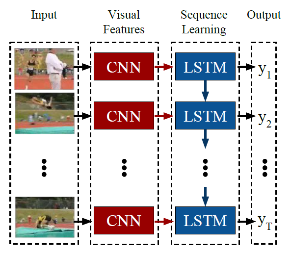

Below, I’ll first describe how to build this model in Keras, then describe two data loading modes: corresponding to variable-length input sequences and fixed-length input sequences respectively.

Building the Model

In actual implementation, when the training dataset is not large, the CNN part can generally use a pre-trained model, then choose whether to fine-tune it. Here I use VGG16 pre-trained on ImageNet, and fine-tune the top 5 layers of VGG16, with other layer parameters unchanged.

Additionally, for each input frame image, the feature map extracted through CNN has size (7,7,512), while LSTM’s input size is (batch_size, timesteps, input_dim). Therefore, we need to convert (7,7,512) to a one-dimensional vector. Here I use the simplest Flatten() method. Actually, more flexible transformations can be used here. For example, the paper Diversified Visual Attention Networks for Fine-Grained Object Classification proposes an attention mechanism to handle these feature maps.

The size of (7,7,512) after direct Flatten is 25088, which is quite large to input directly to LSTM, so a 2048 fully connected layer is added here. This way, the input_dim size for LSTM is 2048.

The key point in the LRCN model is connecting the CNN network part before each LSTM step. In Keras, this can be achieved through the TimeDistributed layer. Also, if variable-length input sequences are needed, the corresponding sequence length parameter should be set to None. In the code below, input_shape is set to (None, 224, 224, 3). None means the input sequence length is variable, while (224, 224, 3) is the fixed input size for pre-trained VGG.

The Keras code for building the model is shown below. To speed up training, LSTM is replaced with GRU:

from keras.applications.vgg16 import VGG16
from keras.models import Sequential, Model
from keras.layers import Input, TimeDistributed, Flatten, GRU, Dense, Dropout
from keras import optimizers

def build_model():
    pretrained_cnn = VGG16(weights='imagenet', include_top=False)
    # pretrained_cnn.trainable = False
    for layer in pretrained_cnn.layers[:-5]:
        layer.trainable = False
    # input shape required by pretrained_cnn
    input = Input(shape = (224, 224, 3))
    x = pretrained_cnn(input)
    x = Flatten()(x)
    x = Dense(2048)(x)
    x = Dropout(0.5)(x)
    pretrained_cnn = Model(inputs = input, output = x)

    input_shape = (None, 224, 224, 3) # (seq_len, width, height, channel)
    model = Sequential()
    model.add(TimeDistributed(pretrained_cnn, input_shape=input_shape))
    model.add(GRU(1024, kernel_initializer='orthogonal', bias_initializer='ones', dropout=0.5, recurrent_dropout=0.5))
    model.add(Dense(categories, activation = 'softmax'))

    model.compile(loss='categorical_crossentropy',
                optimizer = optimizers.SGD(lr=0.01, momentum=0.9, clipnorm=1., clipvalue=0.5),
                metrics=['accuracy'])
    return model

The LSTM parameter initialization above refers to this Zhihu answer: What special tricks do you use when training RNN?. The main points are the choice of initializer method, dropout, and gradient clipping settings. My experiments also confirmed that gradient clipping settings directly affect final accuracy, and the impact is quite significant.

Data Loading

Due to RNN’s structural characteristics, it can accept variable-length inputs, and original image sequence data often also has this characteristic. Therefore, there are two data loading methods. The first is to not process the original data, so each sample’s length may not be the same. The second is to extract a fixed length from each sample.

But the input data shape for both loading methods follows this pattern: (batch_size, sequence_length, width, height, channel)

For the first loading method, according to this issue, there are two handling methods:

Zero-padding
Batches of size 1

Here I use the second handling method, which is setting batch_size to 1, meaning each time only one sample updates the model. Because the second handling method requires setting a fixed length in advance (could be the longest sequence length or length obtained by other means), and padding makes originally shorter sequences longer, which increases memory consumption.

For the second loading method, given a fixed length, we need to extract a fixed-length sequence from the original sequence as “uniformly” as possible, i.e., the interval between frames should be as equal as possible. But this may depend on the specific dataset and task. In my dataset, this approach is reasonable.

Comparison of the two loading methods:

Data storage methods differ. For fixed-length loading, since each sample has the same shape, they can be directly concatenated into a large ndarray, and batch_size can be set to any value during training. But for variable-length loading, we can only take one sample at a time, then add the batch_size dimension through np.expand_dims(imgs, axis=0) (the previous method doesn’t need this because concatenation automatically generates this dimension), then set both batch_size and epoch to 1 when training the model.
Training speed and results differ. First, due to different batch_size, the fixed-length method is faster than the variable-length method, which is easy to understand.

Second, since batch_size is also an important parameter affecting RNN performance, it also affects convergence and results. In my experiments, setting batch_size greater than 1 gives better results.

Implementation code for both loading methods is shown below. It loads data for one sample. The img_dir directory contains all image sequences for one sample, and the sequence sorted by filename is in temporal order.

from collections import deque
from keras.preprocessing import image

def load_sample(img_dir, categories = 7, fixed_seq_len = None):
    label = int(img_dir.split('/')[-2].split('_')[0]) - 1 # extract label from name of sample
    img_names = sorted(os.listdir(img_dir))
    imgs = []
    if fixed_seq_len: # extract certain length of sequence
        block_len = round(len(img_names)/fixed_seq_len)
        idx = len(img_names) - 1
        tmp = deque()
        for _ in range(fixed_seq_len):
            tmp.appendleft(img_names[idx])
            idx = max(idx-block_len, 0)
        img_names = tmp
    for img_name in img_names:
        img_path = img_dir + img_name
        img = image.load_img(img_path, target_size=(224, 224))
        x = image.img_to_array(img)
        imgs.append(x)
    imgs = np.array(imgs)
    label = np_utils.to_categorical(label, num_classes=categories)
    if not fixed_seq_len: # add dimension for batch_size
        #（seq_len, width, height, channel）-> (batch_size, seq_len, width, height, channel)
        imgs = np.expand_dims(imgs, axis=0)
        label = label.reshape(-1, categories)
    return imgs, label

Finally, when designing network architecture, you can verify whether each layer achieves the expected output effect by testing the output size layer by layer. In Keras, you can directly get the output of the current model’s last layer through model.predict(input).

Additionally, while Keras can quickly build models through its provided layers, when more detailed model design is needed, Keras isn’t as suitable. At that point, you’ll need more flexible frameworks like tensorflow/pytorch/mxnet.