Reinforcement Learning Notes (1) - Overview

This article mainly introduces some basic concepts of reinforcement learning: including MDP, Bellman equations, etc., and describes how to transition from MDP to Reinforcement Learning.

Tasks in Reinforcement Learning

Here I’ll use a figure from David Silver’s course, which clearly shows the entire interaction process. This is a modeled representation of human-environment interaction. At each time point, the brain (agent) selects an action \(a_t\) from the available action set A to execute. The environment then gives the agent a reward \(r_t\) as feedback based on the agent’s action, while the agent enters a new state.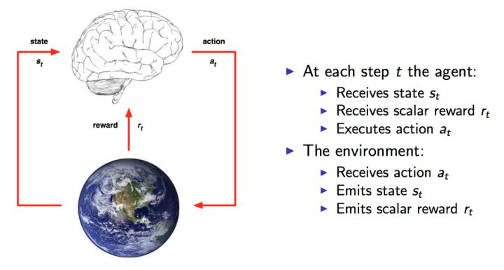

Knowing the entire process, the task objective becomes clear: to obtain as much Reward as possible. More Reward indicates better execution. At each time slice, the agent determines the next action based on the current state. In other words, we need to find an action for a state that maximizes reward. The process from state to action is called a Policy, generally denoted as \(\pi\):

The task of reinforcement learning is to find an optimal Policy such that Reward is maximized.

Initially, we don’t know what the optimal policy is, so we often start with a random policy. Using a random policy for experiments, we can obtain a series of states, actions, and feedback:

\((s_1,a_1,r_1,s_2,a_2,r_2,...s_t,a_t,r_t)\)

This is a series of samples. Reinforcement learning algorithms need to use these samples to improve the Policy, thereby making the Reward in the obtained samples better. Due to this characteristic of making Reward increasingly better, this type of algorithm is called Reinforcement Learning.

MDP (Markov Decision Process)

Reinforcement learning problems can all be modeled as MDP (Markov Decision Process) problems. MDP is actually a model of the environment. The difference between MDP and common Markov chains is the addition of action and reward concepts.

Therefore, a basic MDP can be represented by a five-tuple \((S,A,P,R, \gamma)\), where:

1. \(S\) is a finite set of states
2. \(A\) is a finite set of actions
3. \(P\) is a state transition probability matrix, \(P_a(s, s′)=P(s_{t+1}=s′|s_t=s, a_t=a)\) represents the probability of transitioning to state \(s′\) after executing action \(a\) in state \(s\)
4. \(R\) is a reward function, \(R_a(s, s′)\) represents the immediate reward obtained after transitioning to state \(s′\) by executing action \(a\) in state \(s\)
5. \(\gamma\) is a discount factor, generally in the range [0,1], used to distinguish the importance of current reward versus future reward, generally added before future reward to reduce the weight of future reward.

Therefore, the core problem of MDP is to find a policy \(\pi(s)\) to decide which action to choose in state \(s\). In this case, MDP becomes a Markov chain, and the objective is consistent with the reinforcement learning objective mentioned earlier.

Return and Value Function

The quality of a state is equivalent to the expectation of future returns. Therefore, we introduce Return to represent the return that a state at time t will have:

\(G_t = R_{t+1} + \gamma R_{t+2} + ... = \sum_{k=0}^\infty\gamma^kR_{t+k+1}\)

Above, \(R\) is the Reward feedback, and \(\gamma\) is the discount factor, consistent with the meaning of the symbol in MDP earlier.

From the above equation, unless the entire process ends, we cannot obtain all rewards to calculate the Return for each state. Therefore, we introduce another concept: value function, denoted as \(V(s)\), used to represent the potential future value of a state. By definition, the value function is the expectation of return:

\(V(s) = \mathbb E[G_t|S_t = s]\)

Introducing the value function, we have two methods to achieve the goal of obtaining the optimal Policy:

1. Directly optimize the policy \(\pi(a|s)\) or \(a = \pi(s)\) to make the return higher
2. Estimate the value function to indirectly obtain the optimized policy. The reason is simple - through the value function, we can know the quality of each state, so we know how to choose (e.g., choose the action that maximizes the potential value of the next state), and this choice is the policy we want.

Bellman Equation

When using the second method above to obtain the optimal policy, we need to estimate the Value Function. As long as we can calculate the value function, the optimal decision is obtained. Therefore, the problem becomes how to calculate the Value Function?

According to the earlier definitions of \(G_t\) and \(V(s)\), we have:

\[\begin{align} V(s) & = \mathbb E[G_t|S_t = s]\\\ & = \mathbb E[R_{t+1}+\gamma R_{t+2} + \gamma ^2R_{t+3} + ...|S_t = s]\\\ & = \mathbb E[R_{t+1}+\gamma (R_{t+2} + \gamma R_{t+3} + ...)|S_t = s]\\\ & = \mathbb E[R_{t+1}+\gamma G_{t+1}|S_t = s]\\\ & = \mathbb E[R_{t+1}+\gamma v(S_{t+1})|S_t = s] \end{align}\]

Therefore:

\[\begin{align} V(s) = \mathbb E[R_{t+1} + \gamma V(S_{t+1})|S_t = s] \end{align}\]

This formula is the basic form of the Bellman equation. From the formula, the current state’s value is related to the next step’s value and the current feedback Reward. The implication is that value function calculation can be achieved through iteration.

From MDP to Reinforcement Learning

Returning to the MDP problem, if we know the transition probability \(P\) and reward function \(R\), we can find the optimal policy \(\pi(s)\) through the following method. First, combining the value function and Bellman equation mentioned above:

Formula 1:

\[\begin{align} \pi(s):=\arg \max_a\ \{\sum_{s'}P_{a}(s,s')(R_{a}(s,s')+\gamma V(s'))\} \end{align}\]

Formula 2:

\[\begin{align} V(s) := \sum_{s'}P_{\pi(s)}(s,s')(R_{\pi(s)}(s,s') + \gamma V(s')) \end{align}\]

Formula 1 represents the optimal action to take in state \(s\), and Formula 2 represents the value in state \(s\). We can see that the two are interdependent.

When transition probability \(P\) and reward function \(R\) are known, common methods to solve MDP problems include Value iteration or Policy iteration.

Value Iteration

In Value iteration, the policy function \(\pi\) is not used. The iteration formula is:

\[\begin{align} V_{i+1}(s) := \max_a \sum_{s'} P_a(s,s')(R_a(s,s') + \gamma V_i(s')) \end{align}\]

The subscript \(i\) represents the \(i\)-th iteration. In each iteration round, the value of each state needs to be calculated, and convergence is considered achieved only when the difference between two iteration results is less than a given threshold.

After calculating the converged value function, the policy function \(\pi\) can be obtained through Formula 1. The iteration process is shown below: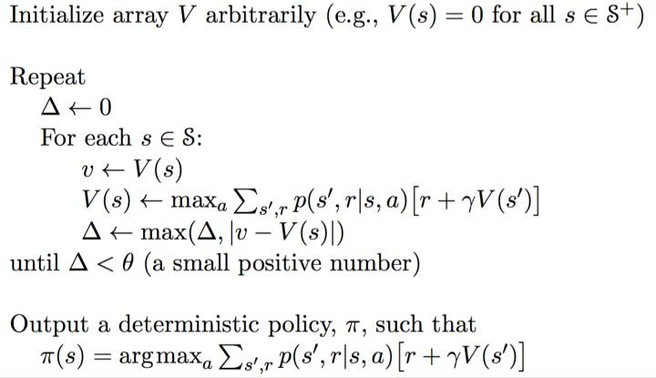

Policy Iteration

Policy iteration simultaneously updates value \(V\) and policy \(\pi\), and can generally be divided into two steps:

1. Policy Evaluation: This is the process of Formula 2 above. The purpose is to update the Value Function until the value converges when the policy is fixed. From another perspective, this is to better estimate the value based on the current policy.
2. Policy Improvement: This is the process of Formula 1 above. Update the policy for each state based on the updated Value Function until the policy stabilizes.

This method essentially uses the current policy (\(\pi\)) to generate new samples, then uses the new samples to better estimate the policy’s value (\(V(s)\)), then uses the policy’s value to update the policy, and repeats. Theory can prove that the final policy will converge to the optimal.

The specific algorithm flow is shown below: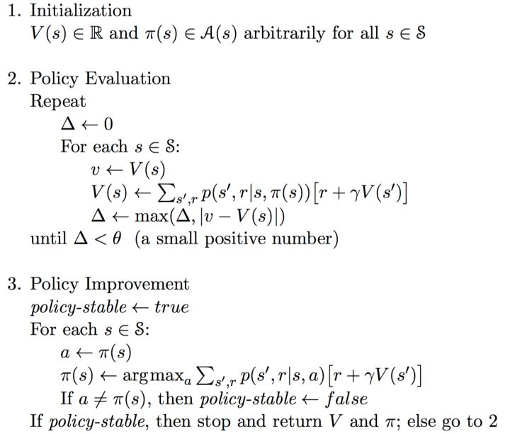

Differences and Limitations

The question arises: what’s the difference between Policy Iteration and Value Iteration, and why is one called policy iteration and the other value iteration?

The reason is actually quite easy to understand. The value \(V\) that policy iteration finally converges to is the value under the current policy (also called evaluating the policy), for the purpose of later policy improvement to get a new policy. So it’s explicitly iterating the policy.

The value that value iteration finally converges to is the optimal value under the current state. When the value finally converges, the optimal policy is obtained. Although policy is implicitly updated in this process, what’s being explicitly updated is value, so it’s called value iteration.

From the above analysis, value iteration is more direct than policy iteration. But the problems are the same - both need to know the transition probability \(P\) and reward function \(R\).

However, for Reinforcement Learning problems, the transition probability \(P\) is often unknown. Knowing the transition probability \(P\) is called having a Model, and this method of obtaining optimal actions through a model is called a Model-based method. But in reality, many problems are difficult to obtain accurate models, so there are Model-free methods to find optimal actions. Methods like Q-learning, Policy Gradient, and Actor Critic are all model-free.

The problem with the earlier methods is needing to know the transition probability \(P\), for the purpose of traversing all possible states after the current state. Therefore, if we adopt a greedy approach, we don’t need to traverse all subsequent states, but directly execute the action with the maximum value state.

Q-learning actually uses this idea. Q-Learning’s basic idea is derived from value iteration, but we need to clarify that value iteration updates all Q values each time, meaning all states and actions. But in fact, in practical situations, we can’t traverse all states and all actions, so we can only get a finite series of samples. The specific algorithm flow will be introduced in detail in the next article.

In summary, this article mainly introduced the tasks and concepts of reinforcement learning, and how to transition from MDP to Reinforcement Learning. In subsequent articles, I will introduce Q-learning methods, Policy gradient methods, and Actor Critic methods that combine both.

References

1. Markov decision process
2. DQN from Introduction to Abandonment 4: Dynamic Programming and Q-Learning
3. Reinforcement Learning Methods Summary