Reinforcement Learning Notes (2) - From Q-Learning to DQN
In the previous article Reinforcement Learning Notes (1) - Overview, I introduced modeling reinforcement learning problems through MDP. However, since reinforcement learning often cannot obtain the transition probabilities in MDP, the value iteration and policy iteration for solving MDP cannot be directly applied to reinforcement learning problems. Therefore, some approximate algorithms have emerged to solve this problem. This article introduces the Q-Learning series methods developed based on value iteration, including Q-Learning, Sarsa, and DQN.
Q-Learning
Q-Learning is a classic algorithm in reinforcement learning. Its starting point is simple: use a table to store the reward that can be obtained by executing various actions in various states. The following table shows two states \(s_1, s_2\), each with two actions \(a_1, a_2\). The values in the table represent rewards:
| - | a1 | a2 |
|---|---|---|
| s1 | -1 | 2 |
| s2 | -5 | 2 |
This representation is actually called Q-Table. Each value inside is defined as \(Q(s, a)\), representing the reward obtained by executing action \(a\) in state \(s\). When choosing, we can adopt a greedy approach, i.e., choose the action with the maximum value to execute.
So the question arises: how to obtain the Q-Table? The answer is to randomly initialize, then continuously execute actions to get environmental feedback and update the Q-Table through the algorithm. Below I’ll focus on how to update the Q-Table through the algorithm.
When we are in a state \(s\) and select action \(a\) based on the Q-Table values, the reward obtained from the table is \(Q(s,a)\). This reward is not the truly obtained reward, but the expected reward. Where is the real reward? We know that after executing action \(a\) and transitioning to the next state \(s'\), we can get an immediate reward (denoted as \(r\)). But besides the immediate reward, we also need to consider the expected future reward of the state \(s'\) we transitioned to. Therefore, the real reward (denoted as \(Q'(s,a)\)) consists of two parts: the immediate reward and the expected future reward. Since future reward is often uncertain, we need to add a discount factor \(\gamma\). The real reward is expressed as follows:
\[\begin{align} Q'(s,a) = r + \gamma\max_{a'}Q(s',a') \end{align}\]
\(\gamma\) is generally set between 0 and 1. Setting it to 0 means only caring about immediate return, setting it to 1 means expected future return is as important as immediate return.
Having the real reward and expected reward, we can naturally think of using the supervised learning approach: calculate the error between the two and update. Q-learning does exactly this. The updated value is the original \(Q(s, a)\), with the update rule:
\[\begin{align} Q(s, a) = Q(s, a) + \alpha(Q'(s, a) - Q(s,a)) \end{align}\]
The update rule is very similar to gradient descent. Here, \(\alpha\) can be understood as the learning rate.
The update rule is simple, but algorithms adopting greedy thinking often have this question: can the algorithm converge, and to a local or global optimum?
Regarding convergence, you can refer to Convergence of Q-learning: a simple proof. This document proves this algorithm can converge. According to this Zhihu question Essential differences between two major RL algorithms? (Policy Gradient and Q-Learning), original Q-Learning theoretically can converge to the optimal solution, but methods approximating Q-Table through Q functions may not converge to the optimal solution (like DQN).
Besides this, Q-Learning also has the Exploration and Exploitation problem. Roughly, it means not always following the currently best-looking solution, but sometimes choosing strategies that don’t look optimal currently, which might explore better strategies faster.
There are many approaches to Exploration and Exploitation. Q-Learning adopts the simplest \(\epsilon\)-greedy: each time, there’s \(\epsilon\) probability of choosing the action with the maximum value in the current Q-Table, and \(1-\epsilon\) probability of randomly choosing a strategy.
The Q-Learning algorithm flow is shown below, image from here: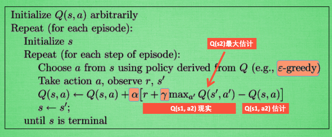
In the above flow, Q-real is the \(Q'(s,a)\) mentioned earlier, and Q-estimate is the \(Q(s,a)\) mentioned earlier.
The following Python code demonstrates the algorithm for updating through Q-Table, referencing code from this repo. The initialization mainly sets some parameters and builds the Q-Table. choose_action selects the current action based on the current state observation using the \(\epsilon\)-greedy strategy; learn updates the current Q-Table; check_state_exist checks if the current state exists in the Q-Table, and creates a corresponding row if not.1
2
3
4
5
6
7
8
9
10
11
12
13
14
15
16
17
18
19
20
21
22
23
24
25
26
27
28
29
30
31
32
33
34
35
36
37
38
39
40
41
42
43import numpy as np
import pandas as pd
class QTable:
def __init__(self, actions, learning_rate=0.01, reward_decay=0.9, e_greedy=0.9):
self.actions = actions # a list
self.lr = learning_rate
self.gamma = reward_decay
self.epsilon = e_greedy
self.q_table = pd.DataFrame(columns=self.actions, dtype=np.float64)
def choose_action(self, observation):
self.check_state_exist(observation)
# action selection
if np.random.uniform() < self.epsilon:
# choose best action
state_action = self.q_table.ix[observation, :]
state_action = state_action.reindex(np.random.permutation(state_action.index)) # some actions have same value
action = state_action.argmax()
else:
# choose random action
action = np.random.choice(self.actions)
return action
def learn(self, s, a, r, s_):
self.check_state_exist(s_)
q_predict = self.q_table.ix[s, a]
if s_ != 'terminal':
q_target = r + self.gamma * self.q_table.ix[s_, :].max() # next state is not terminal
else:
q_target = r # next state is terminal
self.q_table.ix[s, a] += self.lr * (q_target - q_predict) # update
def check_state_exist(self, state):
if state not in self.q_table.index:
# append new state to q table
self.q_table = self.q_table.append(
pd.Series(
[0]*len(self.actions),
index=self.q_table.columns,
name=state,
)
)
Sarsa
Sarsa is very similar to Q-Learning, also making decisions based on Q-Table. The difference lies in the strategy for determining the action to execute in the next state. Q-Learning uses the action with the maximum Q value in the next state when updating the Q-Table for the current state, but the next state may not necessarily choose that action. Sarsa first decides the action to execute in the next state in the current state, and uses the Q value of the action to be executed in the next state to update the current state’s Q value. Sounds confusing, but looking at the flow below will reveal the specific differences between the two. Image from here: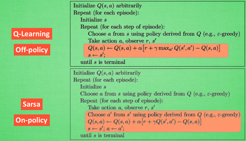
So what’s the difference between these two? This article explains:
This means that SARSA takes into account the control policy by which the agent is moving, and incorporates that into its update of action values, where Q-learning simply assumes that an optimal policy is being followed.
Simply put, Sarsa considers the global situation when executing actions (e.g., determining the next step’s action first when updating the current Q value), while Q-Learning appears more greedy and “short-sighted”, always choosing the action with maximum current benefit (not considering \(\epsilon\)-greedy), without considering other states.
So how to choose? According to this question: When to choose SARSA vs. Q Learning, the conclusion is:
If your goal is to train an optimal agent in simulation, or in a low-cost and fast-iterating environment, then Q-learning is a good choice, due to the first point (learning optimal policy directly). If your agent learns online, and you care about rewards gained whilst learning, then SARSA may be a better choice.
Simply put, if you want online learning while balancing reward and overall strategy (e.g., not too aggressive, agent shouldn’t die quickly), choose Sarsa. If there’s no online requirement, you can find the best agent through Q-Learning offline simulation. That’s why Sarsa is called on-policy and Q-Learning is called off-policy.
DQN
The two methods mentioned earlier both rely on Q-Table. However, when there are many states in the Q-Table, the entire Q-Table might not fit in memory. Therefore, DQN was proposed. DQN stands for Deep Q Network, where Deep refers to deep learning - essentially using a neural network to fit the entire Q-Table.
DQN can solve problems with infinite states and finite actions. Specifically, it takes the current state as input and outputs the Q values for each action. Taking the Flappy Bird game as an example, the input state is nearly infinite (current bird’s position and surrounding pipe positions, etc.), but the output actions are only two (fly or don’t fly). Actually, someone has already used DQN to play this game, see this DeepLearningFlappyBird.
So the core problem in DQN is how to train the neural network. The training algorithm is actually very similar to Q-Learning’s training algorithm, needing to use the difference between Q-estimate and Q-real, then perform backpropagation.
Here’s the algorithm flow from the original paper Playing atari with deep reinforcement learning that proposed DQN: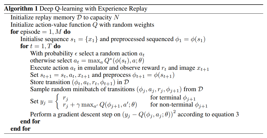
The biggest difference between the above algorithm and Q-Learning is the Experience Replay part. This mechanism actually does repeated experiments first and stores the samples obtained from these experimental steps in memory. Each step is a sample, and each sample is a quadruple including: current state, Q values for various actions in the current state, the immediate reward obtained from the action taken, and Q values for various actions in the next state. With such a sample, we can update the network according to the Q-Learning update algorithm mentioned earlier, except now backpropagation is needed.
The motivation for Experience Replay is that samples constructed in temporal order are related (e.g., \(\phi(s_{t+1})\) above is affected by \(\phi(s_{t})\)) and non-stationary (highly correlated and non-stationary), which easily leads to training results being difficult to converge. Through Experience Replay mechanism’s random sampling of stored samples, this correlation can be removed to some extent, making convergence easier. Of course, this method also has drawbacks - training is in offline form, not online.
Besides this, the action-value function in the algorithm flow above is a deep neural network, because neural networks are proven to have universal approximation capability, meaning they can fit any function. An episode is equivalent to an epoch. The \(\epsilon\)-greedy strategy is also adopted. For code implementation, refer to the FlappyBird DQN implementation above.
The DQN mentioned above is the most primitive network. Later, DeepMind made various improvements, such as Nature DQN adding a new mechanism separate Target Network, which uses another network (Target Network) \(Q'\) instead of network \(Q\) when calculating \(y_j\) in the figure above. The reason is that both calculating \(y_j\) and Q-estimate use the same network \(Q\), which makes samples with large Q also have large y, increasing the possibility of model oscillation and divergence. The reason is still the high correlation between the two. Using another independent network reduces the possibility of training oscillation and divergence, making it more stable. Generally, \(Q'\) directly uses the old \(Q\), e.g., the \(Q\) from 10 epochs ago.
Besides this, the three main methods that significantly improved DQN’s Atari performance are Double DQN, Prioritised Replay, and Dueling Network. I won’t elaborate here. Interested readers can refer to these two articles: DQN from Introduction to Abandonment 6: Various DQN Improvements and Introduction to Deep Reinforcement Learning: RL base & DQN-DDPG-A3C introduction.
In summary, this article introduced value-based methods in reinforcement learning: including Q-Learning and the very similar Sarsa, and also introduced solving the problem of Q-Table being too large due to infinite states through DQN. Note that DQN can only solve problems with finite actions. For infinite actions or actions with continuous values, we need to rely on policy gradient algorithms, which are also the currently more preferred algorithms. The next chapter will introduce Policy Gradient and Actor-Critic methods that combine Policy Gradient and Q-Learning.
References
- Q Learning
- Sarsa
- When to choose SARSA vs. Q Learning
- DQN from Introduction to Abandonment 5: Deep Interpretation of DQN Algorithm
- Introduction to Deep Reinforcement Learning: RL base & DQN-DDPG-A3C introduction