Reinforcement Learning Notes (3) - From Policy Gradient to A3C

In the previous article Reinforcement Learning Notes (2) - From Q-Learning to DQN, we learned that Q-Learning series methods are value-based methods, which compute the value of each state-action pair and then select the action with the maximum value for execution. This is an indirect approach. Is there a more direct method? Yes! That is directly updating the policy. This article introduces Policy Gradient, which is a policy-based method. Additionally, we will introduce the Actor-Critic method that combines policy-based and value-based approaches, as well as DDPG and A3C methods built upon Actor-Critic.

Policy Gradient

Basic Idea

Policy Gradient updates the policy by updating the Policy Network. So what is a Policy Network? It’s actually a neural network where the input is the state and the output is directly the action (not the Q value). The output generally comes in two forms: one is probabilistic, outputting the probability of each action; the other is deterministic, outputting a specific action.

To update the Policy Network, or to use gradient descent to update the network, we need an objective function. For all reinforcement learning tasks, the goal is to maximize the expected cumulative discounted reward, as shown below:

\(L(\theta) = \mathbb E(r_1+\gamma r_2 + \gamma^2 r_3 + ...|\pi(,\theta))\)

This loss function doesn’t seem to have a direct connection with the Policy Network. The reward is given by the environment and has no direct operational relationship with the parameter \(\theta\). So how can we compute the gradient of the loss function with respect to the parameters \(\nabla_{\theta} L(\theta)\)?

The above problem doesn’t provide an update strategy, so let’s think about it from a different angle.

Suppose we have a Policy Network that takes a state as input and outputs action probabilities. After executing an action, we can get a reward or result. At this point, we have a very simple idea: if an action yields more reward, we increase its probability; if an action yields less reward, we decrease its probability.

Of course, using reward to judge the quality of an action is not accurate, and even using result is not accurate (because any reward or result depends on many actions, so we can’t attribute all credit or blame to the current action). However, this gives us a new perspective: if we can construct a good evaluation metric to judge whether an action is good or bad, then we can optimize the policy by changing the probability of actions!

Assuming this evaluation metric is \(f(s,a)\), our Policy Network outputs \(\pi(a|s,\theta)\) as a probability. We can optimize this objective using maximum likelihood estimation. For example, we can construct the following objective function:

\(L(\theta) = \sum log\pi(a|s,\theta)f(s,a)\)

For instance, in a game, if we win, we consider every step in that game as good; if we lose, we consider them as bad. Good \(f(s,a)\) is 1, bad is -1, and we maximize the objective function above.

Actually, besides maximizing the objective function above, we can also directly maximize \(f(s,a)\). As shown in this blog post Deep Reinforcement Learning: Pong from Pixels, directly maximizing \(f(x)\), which is \(f(s, a)\) expectation, yields the same result as the objective function above.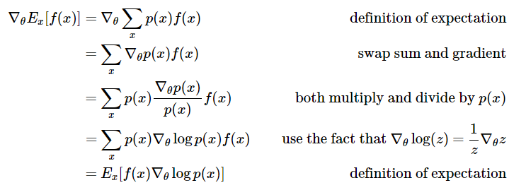

Selection of Evaluation Metric

From the derivation above, we know that in Policy Gradient, how to determine the evaluation metric \(f(s,a)\) is key. We mentioned a simple method above that judges each step in an episode based on whether the episode was won or lost. However, we actually want to get the specific evaluation for each step as we take it, so many other evaluation methods have emerged. For example, this paper High-dimensional continuous control using generalized advantage estimation compares several evaluation metrics.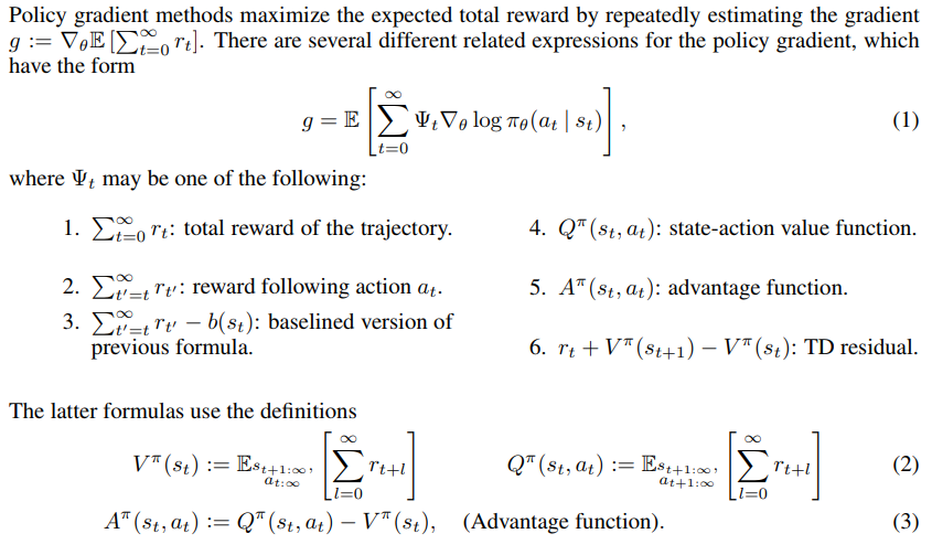

The \(\Psi_t\) in formula (1) above is the evaluation metric at time t. From the figure above, we can see that we can use reward, Q, A, or TD as the evaluation metric for actions. What’s the difference between these methods?

According to this article DRL 之 Policy Gradient, Deterministic Policy Gradient 与 Actor-Critic, the essential difference lies in the variance and bias issue:

Using reward as the action evaluation is the most direct approach. Using the third method in the figure above (reward-baseline) is a common approach. This has low bias but high variance, meaning the reward values are too unstable, which can lead to unstable training.

What about using Q values? Q value is the expected value of reward. Using Q value has lower variance but higher bias. Generally, we choose to use A, Advantage. A=Q-V, is the value of an action relative to the current state. Essentially, V can be seen as a baseline. For the third method above, we can also directly use V as the baseline. However, the same issue exists - A has high variance. To balance variance and bias, using TD is a better approach as it incorporates both the actual reward and the estimated value V. In TD, TD(lambda) balances TD values of different lengths and is a good choice.

In practice, we need to choose different methods based on specific problems. Some problems have rewards that are easy to obtain, while others have very sparse rewards. The sparser the reward, the more we need to use estimated values.

The above is the core idea of Policy Gradient - constructing an objective function through the softmax probability output by the policy network and the obtained reward (through evaluation metrics), then updating the policy network. This avoids the problem where the original reward and policy network are not differentiable. Because of this characteristic of Policy Gradient, many traditional supervised learning problems with discrete softmax outputs can be transformed into Policy Gradient methods. With proper tuning, the results can improve upon supervised learning.

Actor-Critic

The various evaluation metrics mentioned above already encompass the idea of Actor-Critic. The original Policy Gradient often uses episode-based updates, meaning updates only happen after an episode ends. For example, in a game, if the final result is victory, we can consider every step as good; conversely, if it’s a loss, every step is bad. The update process is shown below (image from David Silver’s Policy Gradient slides), and this method is also called Monte-Carlo Policy Gradient.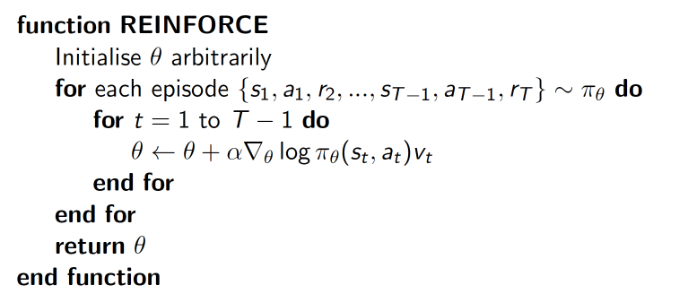

The \(\log \pi_{\theta}(s_t, a_t)\) in the figure is the probability output by the policy network, and \(v_t\) is the result of the current episode. This is the most basic form of policy gradient update. However, this method clearly has problems - a good final result doesn’t mean every step is good. Therefore, an intuitive idea is: can we abandon episode-based updates and use single-step updates instead? Actor-Critic does exactly this.

To use single-step updates, we need to make immediate evaluations for each step. The Critic in Actor-Critic is responsible for this evaluation work, while the Actor is responsible for selecting the action to execute. This is the idea of Actor-Critic. From the various evaluation metrics proposed in the paper above, we can see that Critic’s output can take multiple forms, such as Q value, V value, or TD.

Therefore, the idea of Actor-Critic is to get the evaluation of actions from the Critic module (mostly using deep neural networks), then feed it back to the Actor (mostly using deep neural networks) to let the Actor update its policy. In terms of specific training details, Actor and Critic use different objective functions for updates. You can refer to the code here Actor-Critic (Tensorflow), and the DDPG we’ll discuss next does the same.

Deep Deterministic Policy Gradient(DDPG)

The Policy Gradient mentioned above is still limited to problems with discrete and finite action spaces. However, for problems where the output values are continuous, the above methods don’t work, such as controlling speed in autonomous driving or controlling movement amplitude in robotics.

Initially, this paper Deterministic Policy Gradient Algorithms proposed DPG (Deterministic Policy Gradient) for outputting continuous action values; then the paper Continuous control with deep reinforcement learning improved upon DPG and proposed DDPG (Deep Deterministic Policy Gradient).

We won’t elaborate on DPG here. In short, it mainly proved that the deterministic policy gradient not only exists but is also in a model-free form and is the gradient of the action-value function. Therefore, policy can be represented not only through probability distribution but also extended to infinite action space. For the specific theory, refer to this article 深度增强学习（DRL）漫谈 - 从 AC（Actor-Critic）到 A3C（Asynchronous Advantage Actor-Critic）.

The core improvement of DDPG over DPG is introducing Deep Learning, using deep neural networks to approximate the strategy function \(μ\) and \(Q\) function in DPG, i.e., the Actor network and Critic network; then using deep learning methods to train these neural networks. The relationship between the two is similar to the relationship between DQN and Q-learning.

DDPG’s network structure is Actor network + Critic network. For state \(s\), first get action \(a\) through the Actor network, where \(a\) is a vector; then input \(a\) into the Critic network, which outputs the Q value. The objective function is to maximize the Q value, but the update methods for the two are different. The algorithm flow is shown in the paper: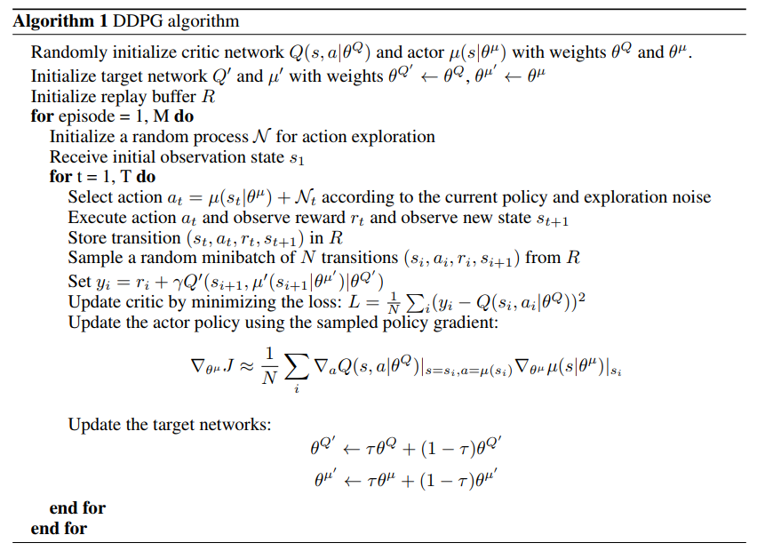

From the algorithm flow, we can see that the Actor network and Critic network are trained separately, but their inputs and outputs are connected. The action output by the Actor network is the input to the Critic network, and the Critic network’s output is used in the Actor network for backpropagation.

The original paper doesn’t give a specific diagram of the two networks. Here’s a diagram from this article. We can see that Critic is similar to the DQN mentioned earlier, but here the input is state + action, and the output is a single Q value rather than Q values for each action.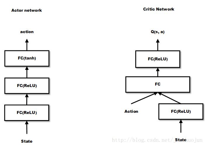

In DDPG, we no longer use a single probability value to represent an action, but use a vector to represent an action. Since vector space can be considered infinite, it can correspond to infinite action space.

Asynchronous Advantage Actor-Critic(A3C)

After proposing DDPG, DeepMind proposed the more effective Asynchronous Advantage Actor-Critic (A3C) on this basis. See the paper Asynchronous Methods for Deep Reinforcement Learning for details.

The A3C algorithm is similar to DDPG, using DNN to fit the policy function and value function estimates. But the differences are:

1. A3C has multiple agents performing asynchronous updates on the network, which brings the benefit of lower correlation between samples, so A3C doesn’t use the Experience Replay mechanism; this allows A3C to support online training mode.
2. A3C has two outputs: one softmax output as the policy \(\pi(a_t|s_t;\theta)\), and one linear output as the value function \(V(s_t;\theta_v)\).
3. The evaluation metric for the Policy network in A3C uses the Advantage Function (i.e., A value) mentioned in the paper that compared multiple evaluation metrics, rather than the simple Q value in DDPG.

The overall structure is shown below (image from this article):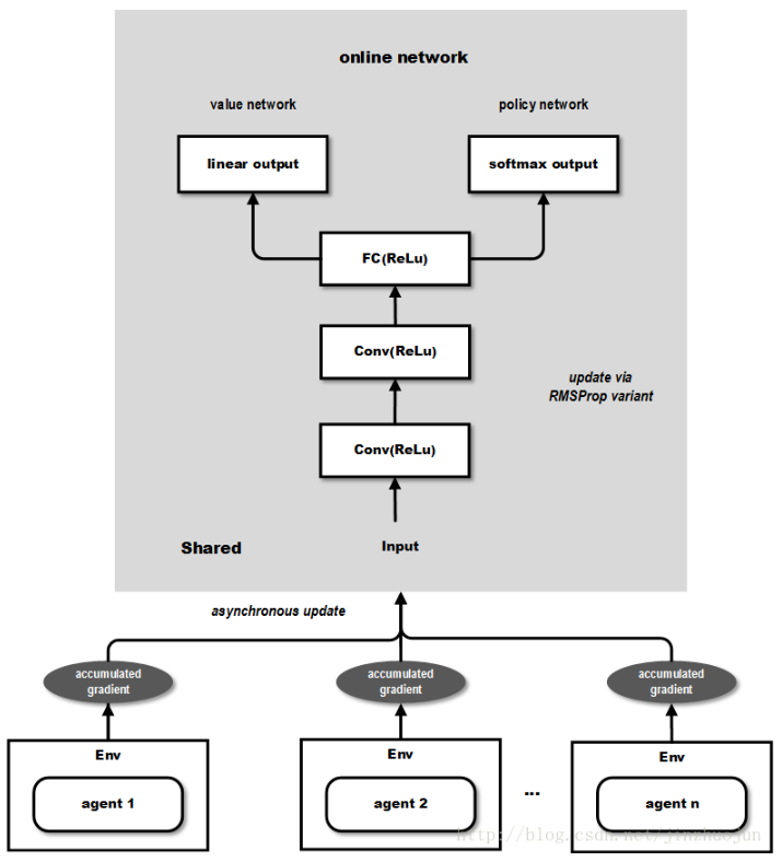

From the above figure, the output contains two parts: the value network part can be used for continuous action value output, while the policy network can be used as probability output for discrete action values, thus able to solve both types of problems mentioned earlier.

The update formulas for the two networks are as follows: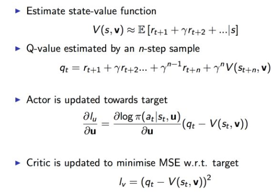

A3C creates multiple agents that execute and learn in parallel and asynchronously in multiple environment instances. A potential benefit is less dependence on GPU or large-scale distributed systems. In fact, A3C can run on a multi-core CPU, and engineering design and optimization are also a focus of this paper.

In summary, this article mainly introduces Policy Gradient methods. The most basic Policy Gradient uses episode-based updates. After introducing Critic, it becomes single-step updates, and this method combining policy and value is called Actor-Critic, where Critic has multiple optional methods. For continuous action outputs, the earlier methods outputting action probability distributions are powerless, so DPG and DDPG were proposed. DDPG’s improvement over DPG is introducing deep neural networks to fit the policy function and value function. On the basis of DDPG, the more effective A3C was proposed, which introduces multiple agents to perform asynchronous updates on the network, not only achieving better results but also reducing training costs.

References

1. 深度增强学习之 Policy Gradient 方法 1
2. Deep Reinforcement Learning: Pong from Pixels
3. 深度增强学习（DRL）漫谈 - 从 AC（Actor-Critic）到 A3C（Asynchronous Advantage Actor-Critic）
4. 深度强化学习（Deep Reinforcement Learning）入门：RL base & DQN - DDPG - A3C introduction