Introduction to CTR Prediction Models - Non-Deep Learning

This article mainly introduces some commonly used models in CTR prediction, focusing on non-deep learning models, including LR, GBDT+LR, FM/FFM, and MLR. Each model will briefly introduce its principles, paper sources, and some open-source implementations.

LR (Logistic Regression)

LR + massive handcrafted features is a long-standing practice in the industry. This method is widely used in the industry due to its simplicity and strong interpretability. However, this approach relies on the effectiveness of feature engineering, which requires deep understanding of specific business scenarios to extract good features.

Principle

LR is a very simple linear model. Its output can be considered as the probability of an event occurring (\(y=1\)), as shown below:

\[\begin{align} h(x) = p(y=1|x) = \sigma(w^Tx+b) \end{align}\]

Where \(w\) is the model parameter, \(x\) is the extracted sample feature, both are vectors, and \(b\) is the bias term. \(\sigma\) is the sigmoid function, i.e., \(\sigma(x) = 1/(1+e^{-x})\)

With the probability of the event occurring, the probability of the event not occurring is \(p(y=0|x) = 1-h(x)\). These two probabilities can be expressed through a single formula:

\[\begin{align} p(y|x) = h(x)^y(1-h(x))^{1-y} \end{align}\]

With this probability value, given \(n\) samples, we can estimate model parameters through maximum likelihood estimation. The objective function is:

\[\begin{align} \max \prod_{i=1}^np(y_i|x_i) \end{align}\]

Usually, we take the log of the probability and add a negative sign to change max to min, rewriting the objective function as:

\[\begin{align} \min -\sum_{i=1}^ny_i\log h(x_i)+(1-y_i)\log (1-h(x_i)) \end{align}\]

The loss function above is also called log loss. In fact, multi-class cross entropy can also be derived through maximum likelihood estimation.

With the loss function, we can solve for optimal parameters through optimization algorithms. Since this is an unconstrained optimization problem, many methods can be used. The most common is gradient descent. Additionally, there are Newton’s method series based on second-order derivatives, ADMM for distributed systems, and the FTRL algorithm proposed by Google in the paper Ad Click Prediction: a View from the Trenches, which is also widely adopted in the industry. This algorithm has good properties of online learning and sparsity. Online learning means its update method is similar to SGD (stochastic gradient descent), and sparsity means the algorithm can solve optimization problems with non-smooth L1 regularization terms. Since this article mainly discusses various CTR prediction models, we won’t expand on optimization algorithms here.

The L1 regularization term mentioned above adds \(C\sum_{i=1}^m |w_i|\) to the original loss function, representing the sum of absolute values of all parameters multiplied by constant \(C\). Adding this term makes most \(|w_i|\) in the final solution equal to 0, which is the origin of the name sparsity. Sparsity reduces model complexity, alleviates overfitting, and has feature selection capability. Since the LR model can be understood as weighted summation of features, if certain feature weights \(w_i\) are 0, these features can be considered unimportant. In CTR prediction, the input is massive handcrafted features, so adding L1 regularization is even more necessary.

Since the L1 regularization term is no longer a smooth differentiable function everywhere, the original gradient descent cannot be directly used when optimizing the loss function. Instead, we need to use the subgradient method or the FTRL algorithm mentioned earlier.

The above covers the basic principles of the LR model. In CTR prediction, the key to applying the LR model lies in feature engineering. The LR model is suitable for high-dimensional sparse features. For categorical features, they can be made high-dimensional and sparse through one-hot encoding. For continuous features, they can first be divided into intervals to become categorical features and then one-hot encoded. Feature combination/crossing is also needed to obtain more effective features.

Some Issues

During the introduction, we used some conclusions directly. Below we explain some of these conclusions:

1. Why can LR’s output be considered as a probability value?

This part involves knowledge of Generalized Linear Models (GLM, Generalized linear model). We’ll skip the complex derivation and give the conclusion directly. Simply put, LR is actually a generalized linear model, whose assumption is that in binary classification \((y|x,\theta)\) follows a Bernoulli distribution (binomial distribution), i.e., given input sample \(x\) and model parameters \(\theta\), whether the event occurs follows a Bernoulli distribution. Assuming the parameter of the Bernoulli distribution is \(\phi\), then \(\phi\) can be used as the click-through rate. Through the derivation of generalized linear models, we can derive that \(\phi\) has the following form:

\[\begin{align} \phi = 1/(1+e^{-\eta}) \end{align}\]

From the above equation, we know that the sigmoid function in LR doesn’t come out of nowhere, and \(\eta\) in the equation is also called the link function, which is an important part of determining a GLM. In LR, it’s a simple linear weighting.

Additionally, if we assume the distribution of the error between the output value and the true value is Gaussian, we can derive Linear Regression from GLM. For detailed derivation of GLM, refer to this article 广义线性模型（GLM）.

2. Why does L1 regularization bring sparsity?

There’s a very intuitive answer here: l1 相比于 l2 为什么容易获得稀疏解？. Simply put, when the absolute value of the derivative of the loss function without regularization term for a certain parameter \(w_i\) is less than the constant \(C\) in the L1 regularization term, the optimal solution for this parameter \(w_i\) is 0.

Because when solving for a certain parameter \(w_i\) to minimize the loss function, we can discuss two cases (where \(L\) is the loss function without regularization term): 1) When \(w_i<0\), the derivative of \(L+C|w_i|\) is \(L'- C\) 2) When \(w_i>0\), the derivative of \(L+C|w_i|\) is \(L'+C\)

When \(w_i<0\), let \(L'- C < 0\), the function is decreasing; when \(w_i>0\), let \(L'+C > 0\), the function is increasing. Then \(w_i=0\) is the optimal solution that minimizes the loss function. Combining \(L'- C < 0\) and \(L'+C > 0\), we get \(C > |L'|\). This is the conclusion we obtained above. This is for a certain parameter, but it can also be extended to all parameters. In fact, the same conclusion can be obtained when solving this problem through subgradient descent.

3. Why do continuous features need to be discretized?

Refer to this question: 连续特征的离散化：在什么情况下将连续的特征离散化之后可以获得更好的效果？

There are several benefits after discretization:

1. Sparse vector inner product multiplication is fast, and calculation results are easy to store
2. Discretized features have strong robustness to outliers: for example, if a feature is age>30 is 1, otherwise 0. If the feature isn’t discretized, an outlier “age 300” would cause great interference to the model;
3. Logistic regression is a generalized linear model with limited expression power; after single variable discretization into N variables, each variable can have its own weight through one-hot encoding, equivalent to introducing non-linearity to the model, improving expression power and fitting capability;
4. After discretization, feature crossing can be performed, changing from M+N variables to M*N variables, further introducing non-linearity and improving expression power;
5. After feature discretization, the model is more stable. For example, if user age is discretized, 20-30 as an interval, a user won’t become a completely different person just because they aged one year. Of course, samples at interval boundaries would be the opposite, so how to divide intervals depends on specific scenarios.

4.1 Why should categorical features be one-hot encoded before input to LR?

Refer to this article One-Hot 编码与哑变量. Simply put, LR modeling requires features to have linear relationships, but in practice few satisfy this assumption, so LR model results are hard to meet application requirements. But by one-hot encoding discrete features, LR can set a weight for each possible value of a feature, enabling more accurate modeling and more precise models. One-hot encoding also performs min-max normalization, overcoming scale differences between different features and making the model converge faster.

Open-source Implementations

Due to the widespread use of LR models, basically every machine learning library or framework has related implementations. For example, sklearn provides a single-machine implementation, spark provides a distributed version implementation, Tencent’s open-source Parameter Server Angel also provides LR+FTRL implementation. Angel supports Spark and is still under development. Besides these, there are many personal open-source implementations on Github, which we won’t list here.

LS-PLM (Large Scale Piece-wise Linear Model)

LS-PLM (also called MLR, Mixture of Logistics Regression) was disclosed by Alibaba’s mom in 2017 in the paper Learning Piece-wise Linear Models from Large Scale Data for Ad Click Prediction, but the model was already used internally at Alibaba’s mom since 2012. This model extends LR to solve the problem that a single LR cannot perform non-linear separation.

Principle

LR is a linear model that generates a linear separation plane in data space, but for non-linearly separable data, this single separation plane obviously cannot correctly separate the data. Taking the figure below as an example (from the paper above), A) shows the distribution of positive and negative samples of a set of non-linear training data; for this problem, LR will generate the separation plane in B), while C) shows the LS-PLM model achieving better results.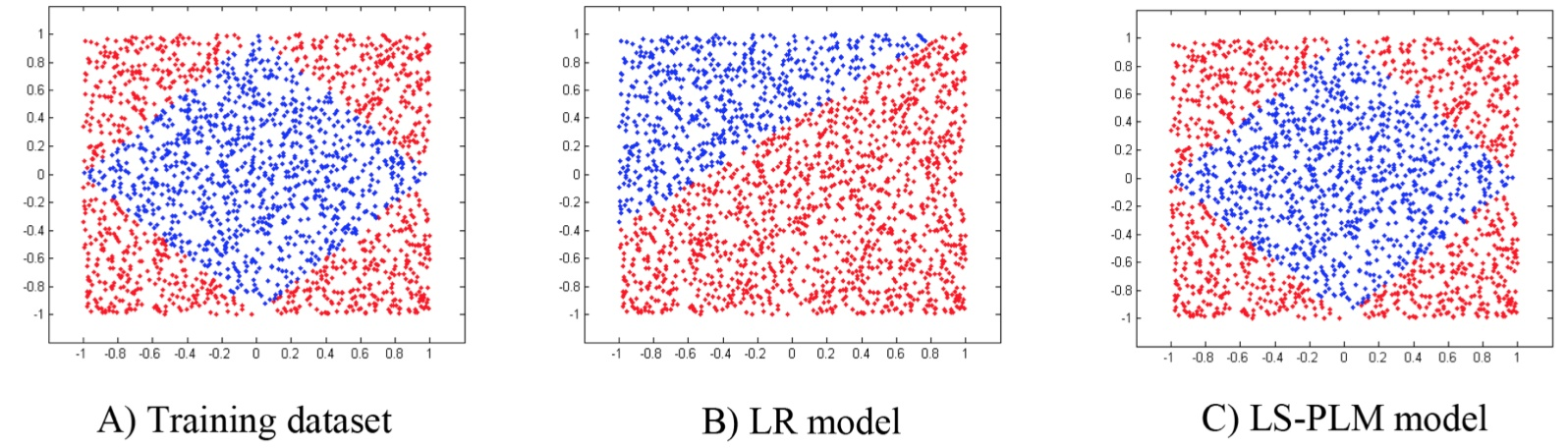

In CTR problems, dividing scenarios for separate modeling is a common approach. For example, for the same product on PC/APP platforms, user usage time and habits may differ significantly; PC might be used more during office hours, while mobile phones are used more during commute or before sleep. If “hour” is a feature, then “hour=23” has more information value for APP but may not mean much for PC. Therefore, distinguishing PC/APP for separate modeling may improve results.

LS-PLM also uses this idea, but here it’s not dividing scenarios but dividing data, by dividing data into different regions, then building LR for each region.

Note that a sample is not uniquely assigned to one region, but distributed to different regions by weight. The idea is similar to LDA (Latent Dirichlet allocation) where a word is distributed to multiple topics by probability.

The formula in the paper is:

\[\begin{align} p(y=1|x) = g ( \sum_{j=1}^m \sigma(\mu_j^T x)\eta(w_j^Tx)) \end{align}\]

The symbols in the formula are defined as follows:

Parameter definitions: - \(m\): number of regions (hyperparameter: generally 10~100) - \(\Theta=\{\mu_1,\dots,\mu_m, w_1,\dots,w_m \}\): model parameters to be trained - \(g(\cdot)\): function to make the model conform to probability definition (probability sums to 1) - \(\sigma(\cdot)\): function to distribute samples to regions - \(\eta(\cdot)\): function to separate samples within a region

The formula proposed earlier is more like a framework. In the paper, only the case where \(g(x) = x\), \(\sigma\) = softmax, \(\eta\) = sigmoid is discussed. Therefore, the above formula can be written as:

\[\begin{align} p(y=1|x) = \sum_{i=1}^m \frac{e^{\mu_i^Tx}}{\sum_{j=1}^m e^{\mu_j^Tx}}\frac{1}{1+e^{-w_i^Tx}} \end{align}\]

This formula has actually become a bagging mode of weighted summation through multiple LR models, but here the weight of each model is learned rather than predetermined.

With the probability function, the subsequent derivation is the same as LR earlier - first get the \(\max\) problem through maximum likelihood estimation, then add a negative sign to convert to the \(\min\) problem for the loss function. We won’t derive this in detail here.

In LS-PLM, regularization terms are also needed. Besides the L1 regularization mentioned in LR, the paper also proposes the \(L_{2,1}\) regularization term, expressed as:

\[\begin{align} ||\Theta||_{2,1} = \sum_{i=1}^d \sqrt {\sum_{j=1}^m(\mu_{ij}^2+w_{ij}^2)} \end{align}\]

Where \(d\) represents the feature dimension, and \(\sqrt {\sum_{j=1}^m(\mu_{ij}^2+w_{ij}^2)}\) represents L2 regularization for all parameters of a certain feature dimension, while the outer \(\sum_{i=1}^d\) represents L1 regularization for all features. Since the value after square root must be positive, no absolute value is needed here. Because it combines L1 and L2 regularization terms, the paper calls this the \(L_{2,1}\) regularization term.

Since both the loss function and regularization term are smooth and differentiable, optimization is simpler than LR with L1 regularization, and more optimization methods are available.

MLR is suitable for the same scenarios as LR, also suitable for high-dimensional sparse features as input.

Open-source Implementations

The Tencent PS Angel mentioned earlier implements this algorithm, see here; Angel is developed in Scala. There are also personal open-source versions like alphaPLM, written in C++. If implementation is needed, you can refer to the above materials.

GBDT+LR (Gradient Boost Decision Tree + Logistic Regression)

GBDT + LR was proposed by Facebook in the paper Practical Lessons from Predicting Clicks on Ads at Facebook. The idea is to use GBDT to help us do part of the feature engineering, then use GBDT’s output as LR’s input.

Principle

Whether LR or MLR mentioned earlier, massive feature engineering is unavoidable. For example, conceiving possible features, discretizing continuous features, one-hot encoding discretized features, and finally performing second-order or third-order feature combination/crossing. The purpose is to obtain non-linear features. But feature engineering has several difficulties:

1. How to select split points for continuous variables?
2. How many parts to discretize into is reasonable?
3. Which features to cross?
4. How many orders of crossing - second, third, or more?

In the GBDT + LR model, GBDT takes on the feature engineering work. Let’s first introduce GBDT.

GBDT was first proposed in the paper Greedy Function Approximation：A Gradient Boosting Machine; GBDT has two main concepts: GB (Gradient Boosting) and DT (Decision Tree). Gradient Boosting is a form of boosting in ensemble learning, and Decision Tree is a type of model in machine learning. We won’t expand on these two, only describing what’s used in GBDT. For introduction to decision trees, refer to this article 决策树模型 ID3/C4.5/CART 算法比较.

In GBDT, the decision tree used is CART (Classification And Regression Tree), used as a regression tree. This regression tree sets a value for a certain feature at each tree node during splitting. If the sample’s corresponding feature value is greater than this given value, it belongs to one subtree; if less, it belongs to another subtree.

Therefore, the key problem in building a CART regression tree is selecting the specific feature and the specific value on that feature. The selection criterion is minimizing squared error. For any split, the squared error is calculated as follows:

1. Suppose after splitting, the left subtree has \(m\) samples, the right subtree has \(n\) samples
2. Calculate the mean of target values in the left subtree as \(y_m = \frac{1}{m}\sum_{i=1}^{m}y_i\), similarly calculate the mean of target values in the right subtree as \(y_n = \frac{1}{n}\sum_{j=1}^{n}y_j\)
3. The sum of squared errors is \(L = \sum_{i=1}^m(y_i - y_m)^2 + \sum_{j=1}^n(y_j - y_n)^2\)
4. For each possible split value, we can calculate its squared error sum \(L\), and choose the split point that minimizes \(L\).

The above is the “DT” part in GBDT, used to solve a regression problem. Given a set of samples, we can build a CART to fit these samples through the above method. Now let’s talk about the “GB” part in GBDT.

Simply put, gradient boosting is stacking the outputs of several models as the final model output. The figure below shows a simple example (from the paper proposing xgb: XGBoost: A Scalable Tree Boosting System):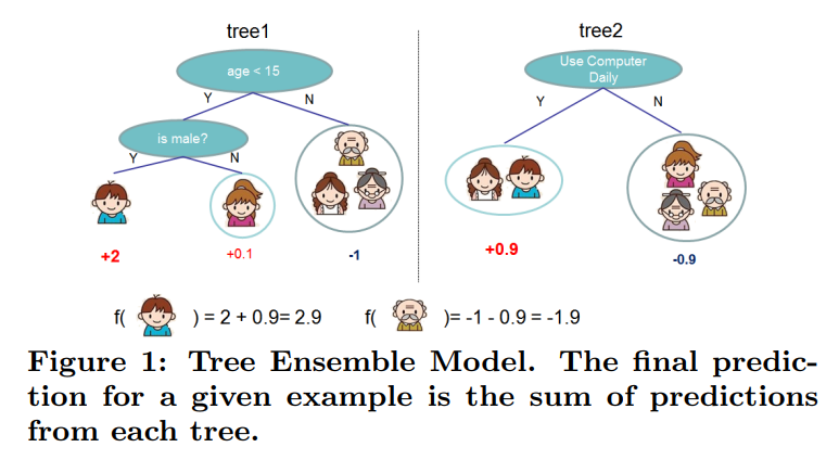

The equation below stacks \(T\) \(f_t(x)\) models as the final model. In GBDT, \(f_t(x)\) is a CART, though \(f_t(x)\) is not limited to tree models.

\[\begin{align} F(x) = \sum_{t=1}^Tf_t(x) \end{align}\]

When building each tree, the difference in input samples is the target value \(y\) for each sample. When building the \(k\)-th tree, for the original sample \((x_i, y_i)\), its target value becomes:

\[\begin{align} y_{ik} = y_i - \sum_{t=1}^{k-1}f_t(x_i) \end{align}\]

So the input to the \(k\)-th tree becomes \((x_i, y_{ik})\). Therefore, when building the \(k\)-th tree, we’re actually fitting the residual between the sum of outputs of the first \(k-1\) trees and the sample’s true value.

Returning to our GBDT + LR model, we first train a batch of tree models through GBDT as mentioned earlier. Then when a sample is input to each tree, it ultimately falls into a specific leaf node. We mark this node as 1 and other leaf nodes as 0. This way, each tree’s output is equivalent to a one-hot encoded feature. The figure below is from Facebook’s original paper, showing two trees. If input \(x\) falls into the first leaf node in the first tree and the second leaf node in the second tree, then the feature input to LR is [1, 0, 0, 0, 1].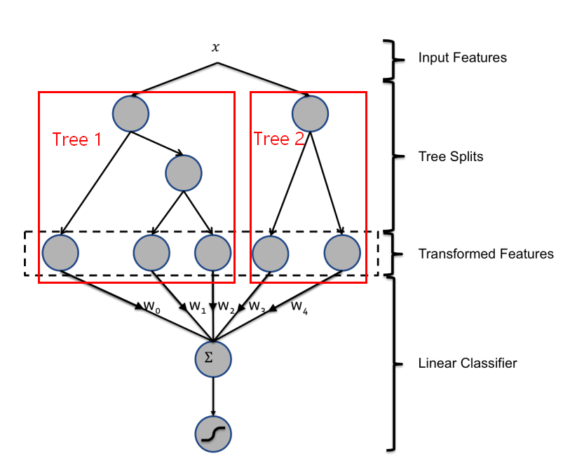

In the GBDT+LR approach, each decision tree’s path from root node to leaf node passes through different features. This path is a feature combination, including second-order, third-order, or even higher. Therefore, the output one-hot features are the result of original feature crossing. Each feature dimension can actually be traced back to its meaning because the path from root to leaf node is unique. Falling into a certain leaf node means this feature satisfies all node judgment conditions in that path.

GBDT is suitable for the opposite problem type as LR. GBDT is not suitable for high-dimensional sparse features because this easily leads to a large number and depth of trained trees, causing overfitting. Therefore, features input to GBDT are generally continuous features.

In CTR prediction, there are many ID features. For such discrete features, there are generally two approaches: 1) Discrete features are not directly input to GBDT for encoding, but are one-hot encoded and directly input to LR; for continuous features, first discretize and feature cross through GBDT to output one-hot encoded features, then combine these two types of one-hot features and directly input to LR. The general framework is shown below: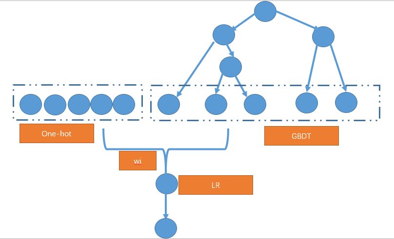

2. Input discrete features to GBDT for encoding, but only keep those high-frequency discrete features. This way, the dimension of one-hot features input to GBDT decreases, and GBDT also performs combination and crossing of original one-hot features.

Some Issues

1. Where does the gradient in GBDT appear?

After all this derivation, we haven’t mentioned gradient. Actually, gradient information is already used when fitting residuals.

First, we need to shift our thinking. The gradient descent we usually use in optimization is for a certain parameter, or in parameter space. But besides parameter space, we can also work in function space. The figure below compares the two approaches (both images from GBDT 算法原理与系统设计简介):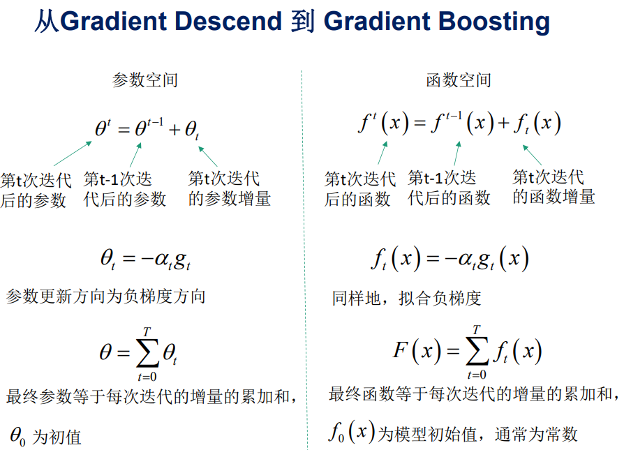

In function space, we directly take derivatives of functions. Therefore, the GBDT algorithm flow is: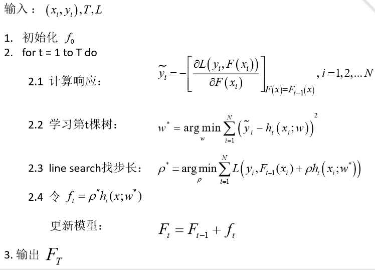

The \(\tilde{y_i}\) in the figure above is the residual of the \(i\)-th sample we mentioned earlier. When the loss function is squared loss, i.e., \[L(y,F(x)) = \frac{1}{2}(y-F(x))^2\]

The residual obtained by taking the derivative with respect to \(F(x)\) is:

\[\begin{align} \tilde{y_i} = y_i - F(x_i) \end{align}\]

This is exactly the difference between the sample’s true value and the sum of outputs of previously built trees we mentioned earlier. If the loss function changes, this residual value will also change accordingly.

2. How does GBDT handle classification problems?

The GBDT we discussed above handles regression problems. But for CTR prediction, broadly speaking, it’s a classification problem. How does GBDT handle this?

In regression problems, each iteration of GBDT builds a tree, essentially building a function \(f\). When the input is x, the tree’s output is \(f(x)\).

In multi-classification problems, assuming there are \(k\) classes, each iteration essentially builds \(k\) trees. For a sample \(x\), the predicted values are \(f_{1}(x), f_{2}(x), ..., f_{k}(x)\).

Here, mimicking multi-class logistic regression, we use softmax to produce probabilities. The probability of belonging to class \(j\) is:

\[\begin{align} p_{c} = \frac{\exp(f_{j}(x))}{ \sum_{i=1}^{k}{exp(f_{k}(x))}} \end{align}\]

Through the above probability values, we can calculate the log loss for each class. According to the GBDT derivation in function space above, we can calculate a gradient for \(f_1\) to \(f_k\), which is the current round’s residual for the next iteration to learn. That is, each iteration simultaneously produces k trees.

When making final predictions, input \(x\) gets \(k\) output values, then obtain the probability of each class through softmax.

For more detailed derivation, refer to this article: 当我们在谈论 GBDT：Gradient Boosting 用于分类与回归

Open-source Implementations

There are few open-source solutions that directly implement GBDT + LR, but since the two have weak coupling, we can first train GBDT, then transform original features through GBDT and feed to LR. GBDT has multiple efficient implementations, such as xgboost and LightGBM.

FM (Factorization Machine)

FM (Factorization Machine) was proposed in 2010 in the paper Factorization Machines, aiming to solve the feature combination problem under sparse data. The idea is to perform matrix decomposition on the parameter matrix composed of combination feature parameters, thereby obtaining the latent vector representation of each original feature. Updating feature latent vectors is robust to data sparsity. For FM and FFM, Meituan’s article: 深入 FFM 原理与实践 has already written very detailedly. This article mainly references that article for modification.

Principle

FM can be considered as adding second-order feature combination on top of LR, meaning at most two features are multiplied. The model can be expressed as:

\[\begin{align} y(\mathbf{x}) = w_0+ \sum_{i=1}^n w_i x_i + \sum_{i=1}^n \sum_{j=i+1}^n w_{ij} x_i x_j \end{align}\]

From the model, we can see that FM is LR with an added final second-order cross term.

From the formula above, we can see there are \(\frac{n(n−1)}{2}\) combination feature parameters, and any two parameters are independent. However, in practical application scenarios where data sparsity widely exists, training second-order parameters is very difficult, because training each parameter \(w_{ij}\) requires a large number of samples where both \(x_i\) and \(x_j\) are non-zero; due to sample data being already sparse, samples satisfying both \(x_i\) and \(x_j\) non-zero will be very few. Insufficient training samples will lead to inaccurate parameter \(w_{ij}\), ultimately seriously affecting model performance.

How to solve this problem? FM borrows the idea of matrix decomposition. In recommendation systems, we perform matrix decomposition on the user-item matrix, so each user and each item gets a latent vector. As shown below: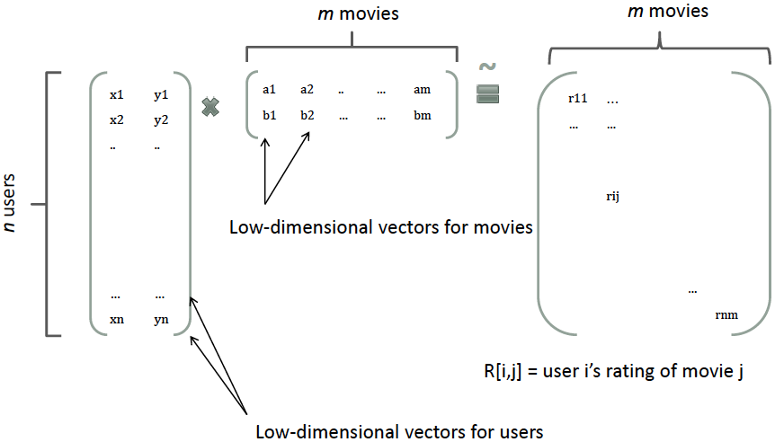

Similarly, all second-order parameters \(w_{ij}\) can form a symmetric matrix \(W\), which can be decomposed as \(W=V^TV\). The \(j\)-th column of \(V\) is the latent vector of the \(j\)-th feature. In other words, each parameter can be expressed as the inner product of two latent vectors, i.e., \(w_{ij}=<v_i,v_j>\), where \(v_i\) represents the latent vector of the \(i\)-th feature. This is the core idea of the FM model. Therefore, the equation above can be rewritten as:

\[\begin{align}y(\mathbf{x}) = w_0+ \sum_{i=1}^n w_i x_i + \sum_{i=1}^n \sum_{j=i+1}^n <v_i, v_j>x_i x_j \end{align}\]

Assuming the latent vector length is \(k(k<<n)\), the number of second-order parameters reduces to \(kn\), far fewer than the polynomial model. Additionally, parameter factorization makes the parameters of \(x_hx_i\) and \(x_ix_j\) no longer independent, so we can relatively reasonably estimate FM’s second-order parameters under sparse samples.

Specifically, the coefficients of \(x_hx_i\) and \(x_ix_j\) are \(<v_h,v_i>\) and \(<v_i,v_j>\) respectively, with a common term \(v_i\). That is, all samples containing non-zero combination features of \(x_i\) (i.e., there exists some \(j≠i\) such that \(x_ix_j≠0\)) can be used to learn the latent vector \(v_i\), which largely avoids the impact of data sparsity. In the polynomial model, \(w_{hi}\) and \(w_{ij}\) are independent.

Additionally, the original paper optimized the time complexity of calculating feature cross terms. See the formula below:

\[\begin{align} \sum_{i=1}^n \sum_{j=i+1}^n \langle \mathbf{v}_i, \mathbf{v}_j \rangle x_i x_j = \frac{1}{2} \sum_{f=1}^k \left(\left( \sum_{i=1}^n v_{i, f} x_i \right)^2 - \sum_{i=1}^n v_{i, f}^2 x_i^2 \right) \end{align}\]

From the formula, we know the original computational complexity is \(O(kn^2)\), while the improved time complexity is \(O(kn)\).

In CTR prediction, applying sigmoid transformation to FM’s output is consistent with Logistic Regression, so the loss function solving methods and optimization algorithms are basically the same. We won’t elaborate on this.

Since FM can be seen as LR with added second-order feature combination, and the model itself has good robustness to sparsity, FM’s applicable range is the same as LR, both suitable for high-dimensional sparse features as input.

Open-source Implementations

FM has single-machine open-source implementations on github: fastFM and pyFM. fastFM is an academic project that published related paper fastFM: A Library for Factorization Machines, extending FM. The Tencent PS Angel mentioned earlier also implements this algorithm, see here.

FFM (Field-aware Factorization Machine)

FFM was published in the paper Field-aware Factorization Machines for CTR Prediction, proposed by students from National Taiwan University when participating in 2012 KDD Cup. This paper borrowed the field concept from the paper Ensemble of Collaborative Filtering and Feature Engineered Models for Click Through Rate Prediction, proposing the upgraded version model FFM of FM.

Principle

By introducing the concept of field, FFM groups features of the same nature into the same field. Simply put, numerical features generated from one-hot encoding of the same categorical feature can be placed in the same field, including user gender, occupation, category preference, etc.

In FFM, for each feature dimension \(x_i\), a latent vector \(v_{i,f_j}\) is learned for each field \(f_j\) of other features. Therefore, latent vectors are not only related to features but also to fields. That is, assuming there are \(f\) fields, each feature has \(f\) latent vectors, using different latent vectors when combining with features of different fields, while in the original FM, each feature has only one latent vector.

Actually, FM can be seen as a special case of FFM, which is the FFM model when all features belong to one field. Based on FFM’s field-aware property, we can derive its model equation as:

\[\begin{align} y(\mathbf{x}) = w_0 + \sum_{i=1}^n w_i x_i + \sum_{i=1}^n \sum_{j=i+1}^n \langle \mathbf{v}_{i, f_j}, \mathbf{v}_{j, f_i} \rangle x_i x_j \end{align}\]

Where \(f_j\) is the field that the \(j\)-th feature belongs to. If the latent vector length is \(k\), then FFM’s second-order parameters are \(nfk\), far more than FM’s \(nk\). Additionally, because latent vectors are field-related, FFM’s second-order term cannot be simplified, and its prediction complexity is \(O(kn^2)\).

Actually, FFM is a more detailed classification on top of FM, increasing the number of parameters to make the model more complex and able to fit more complex data distributions. But the derivation of the loss function and optimization algorithms are the same as FM and LR earlier, so we won’t repeat.

FFM is suitable for the same scenarios as FM and LR, suitable for high-dimensional sparse features as input.

Open-source Implementations

FFM’s earliest open-source implementation is libffm provided by National Taiwan University. Last year, xLearn also provided implementation of this algorithm, with more friendly API than libffm.

Additionally, since FM/FFM can be seen as enhanced versions of LR with feature crossing, they have the same requirements for input feature characteristics. Therefore, the GBDT+LR above can also be directly applied to GBDT+FM/FFM. It’s worth mentioning that students from National Taiwan University won the competition hosted by Criteo in 2014 using GBDT+FFM. For implementation details, refer to kaggle-2014-criteo.

Summary

In non-deep learning, we can see that mainstream models are basically extensions of LR or combinations of LR with other models. The reason is that LR is simple, has good theoretical foundation, strong interpretability, can obtain importance of each feature, and can directly output probability values. But the unavoidable and most important part in applying LR is manual feature engineering. Features determine the upper bound. Although FM/FMM and GBDT+LR to some extent play the role of automatic feature engineering, manual features still account for the majority.

The deep learning methods we’ll discuss next can to some extent alleviate this problem, because deep learning can automatically learn effective features through the model. Therefore, deep learning is also classified as a type of representation learning. However, there’s no free lunch - the convenience of feature engineering brings uninterpretability of features. So the choice still depends on specific needs and business scenarios.