Reading Notes on "Forecasting High-Dimensional Data"

Posted on 2018-11-15 标签计算广告 , 机器学习

“Forecasting High-Dimensional Data” is a paper by Yahoo! about traffic forecasting. In guaranteed advertising, it’s necessary to forecast the traffic volume for specific targeting in advance for reasonable selling and allocation. However, since there are many combinations of targeting (due to diverse advertiser needs), and engineering constraints don’t allow forecasting traffic for every possible targeting, this paper proposes to first forecast traffic for some basic targeting, then calculate traffic for various targeting combinations through a correlation model. This approach is highly practical and is also the traffic forecasting method used in the previously mentioned article “Budget Pacing for Targeted Online Advertisements at LinkedIn”.

Problem Definition

Earlier I briefly mentioned the background of the problem this paper addresses. The paper calls a most basic targeting (e.g., gender being male) an attribute, and each advertiser’s required traffic is a combination of several attributes. Therefore, the number of combinations is enormous. The paper aims to effectively forecast traffic for all combinations.

An intuitive approach would be to collect historical data for a combination, then train a model and make forecasts. However, the most fatal problem with this method is that the time required for collecting historical data and model training is intolerable in practice, requiring several hours (the paper requires returning traffic forecasts for a combination within hundreds of milliseconds). Could this be done offline? The answer is also no, because we don’t know which combinations will be used in the future, so all combinations need to be forecasted, and this number is too large.

Solution Approach

The solution proposed in the paper is to first perform the historical statistics and forecasting operations mentioned above on a small representative subset of combinations. These representative traffic can be obtained from historical statistical data (e.g., combinations with the most visits, etc.) or manually selected. Then combined with the correlation model mentioned in the paper, traffic for all combinations can be forecasted from this small subset.

Let me explain the overall solution approach in detail below.

System Overview

The system diagram of the method proposed in the paper is shown below. Each Historical Data Point is actually a historical query containing combinations of certain attributes. This data has two main purposes:

Sent to the Historical Data Aggregator to perform historical statistics on certain representative Selected Attribute Combinations, and make time series forecasts through models. The time series forecasting here uses the SARIMA model.
Used to build the Correlation Model, which together with the forecast results of several Selected Attribute Combinations above, returns forecasts for online queries.

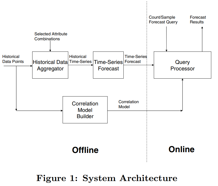
We can see that the focus of the paper is on the construction of the correlation model and how the correlation model works in the online part.

Correlation Model

Earlier I mentioned performing time series forecasting on a subset of representative combinations (the Selected Attribute Combinations in the figure above), denoted as \(Q = \lbrace Q_1, Q_2,... Q_m \rbrace\), called base queries. Then for an online query \(q\), its forecasting steps are as follows:

Select a base query \(Q_k\) from \(Q\) such that \(q \subseteq Q_k\)
Calculate the traffic for \(Q_k\) within future time \(T\), denoted as \(B(Q_k, T)\)
Calculate the probability of \(q\) appearing in \(Q_k\), denoted as \(R(q|Q_k)\)
Return the forecast result for \(q\) as \(B(Q_k, T) \times R(q|Q_k)\)

What the Correlation Model does is step 3: calculating the ratio.

In the first step, there must exist some \(Q_k\) such that \(q \subseteq Q_k\). Why?

Assuming there are n attributes in total, if each attribute is treated as a base query (this gives n base queries in \(Q\)), then any combination of attributes will definitely belong to several base queries in Q. What if more than one \(Q_k\) exists such that \(q \subseteq Q_k\)? In this case, we need to select the smallest \(Q_k\), where smallest means there is no \(Q_l\) that simultaneously satisfies \(q \subseteq Q_l\) and \(Q_l \subseteq Q_k\). For a simple example, if there are two base queries \(Q1 = a_1, Q_2 = a1 \wedge a_2\), then for a query \(q = a1 \wedge a_2 \wedge a_3\), \(Q_2\) should be selected as \(Q_k\).

Below I explain the three correlation models mentioned in the paper.

Full Independence Model (FIM)

FIM is essentially Naive Bayes, assuming each attribute is mutually independent, i.e.:

\[\begin{align} R(Gender = male \wedge Age < 30|Q_k) = R(Gender = male|Q_k) \times R(Age < 30|Q_k) \end{align}\]

This means we only need to calculate the ratio \(R(.| Q_k)\) for each individual attribute of \(Q_k\). The specific calculation method is as follows:

\[\begin{align} R(a_i|Q_k) = \frac{|a_i \in (Q_k \wedge P_t)|}{|Q_k \wedge P_t|} \end{align}\]

Partwise Independence Model (PIM)

Assuming all attributes are mutually independent is obviously unreasonable, because some attributes are correlated, such as age and income generally being related. Therefore, PIM essentially calculates the ratios for certain possibly correlated attributes together. That is:

\[R(Gender = male \wedge Age < 30 \wedge Incom > 10000|Q_k) = R(Gender = male|Q_k) \times R(Age < 30 \wedge Incom > 10000|Q_k)\]

The ratio calculation formula is similar to the above.

Sampling-based Joint Model (SJ M)

The two methods above both assume mutual independence between attributes, which still has certain limitations. Can we completely avoid the independence assumption? The Sampling-based Joint Model (SJ M) proposed in this paper avoids the independence assumption.

Although called a model, the method is still statistics. To avoid too large a quantity, sampling is first performed. The data after sampling is denoted as \(S\), then the number of base query \(|Q_k|\) in \(S\), denoted as \(|Q_k \cap S|\), is calculated. This part is done offline. When a query \(q\) comes online, the number in \(S\) satisfying \(q\) is calculated and denoted as \(n\). The ratio calculation formula is simple:

\[\begin{align} R(q|Q_k) = \frac{n}{|Q_k \cap S|} \end{align}\]

The entire process is conceptually very simple, without involving attributes, so there’s no attribute independent assumption. However, the key problem is how to efficiently calculate the numerator and denominator counts. The paper uses bitmap index, and uses an improved method for bitmap index proposed in the paper Optimizing bitmap indices with efficient compression.

Experimental Results

Data

The experiment used Yahoo!’s partial page historical access data from the past year, with half used for time-series forecasting and half for validation (divided by time). For some combinations, data accumulated over the past four years was used for forecasting. The Correlation Model used data from the past week for training, and SJ M sampled 20 million data points.

Evaluation Metrics

Engineering evaluation metrics include speed and space, i.e., time and space evaluation.

The effectiveness evaluation metric is mainly accuracy, using absolute percentage error (APE). Assuming the forecast value is \(F\) and the true value is \(A\), APE is defined as:

\[\begin{align} APE = \frac{|F-A|}{A} \end{align}\]

APE is for a single query, but we often want to verify the effectiveness of a series of queries. The metric is Root Mean Square Error (RMSE), defined as follows, where \(w_q\) represents the weight of each query, set to the number of times the query appeared in contracts over the past two years:

\[\begin{align} RMSE = \sqrt{\frac{\sum_{q \in Q}w_qAPE^2(q)}{\sum_{q \in Q}w_q}} \end{align}\]

Results Comparison

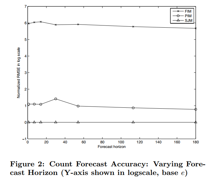
Below is the RMSE (logarithm taken) comparison of the three models. The forecast horizon on the x-axis indicates the effect when forecasting how many days into the future. We can see that assuming attribute independence reduces the final effect.

Additionally, the time for each model to return results online is less than 50 milliseconds; and the memory usage of FIM and PIM models is about 500 MB, because these two models only need to store ratio values and forecast trend curves. However, SJ M’s memory reaches about 20GB (20 million data points), with space mainly consumed by the bitmap index.