Overview of EE (Exploitation-Exploration) Problem

Posted on 2019-01-05 标签计算广告 , 机器学习

The EE (Exploitation & Exploration) problem is very common in computational advertising/recommender systems. More broadly, any decision-making problem involves the EE problem. Simply put, this problem addresses whether to choose the optimal strategy based on existing experience (Exploitation) or explore new strategies to improve future returns (Exploration) when making decisions. This article mainly introduces three common methods to solve this problem: random methods, UCB methods, and Thompson sampling methods, focusing on the specific procedures and basic ideas of each method.

MAB Modeling

The EE problem is typically modeled through MAB (Multi-Armed Bandit). As shown below, all arms represent the choices available in each decision, and pulling an arm represents making the corresponding choice.

The symbolic representation of MAB is as follows:

MAB can be represented as a tuple <$A, R$>
$A$ represents a set of possible actions, and $R(r|a)$ represents the reward distribution given an action
At each moment, action $a_t$ is selected from $A$ according to a given strategy, and the environment generates reward $r_t$ based on distribution $R(r|a)$
The goal is to maximize the sum of rewards $\sum_{t=1}^T r_t$

The strategy in step 3 above is the solution method for the EE problem discussed below. Except for random methods, both UCB methods and Thompson sampling methods work by defining the expected reward for each arm, then selecting the arm with the maximum expected reward. UCB follows the frequentist approach, believing that each arm’s expected reward is fixed. Through experimental records, we obtain its historical reward situation, then add a bound to form the expected reward. Thompson sampling follows the Bayesian approach, believing that the arm’s expected reward follows a specific probability distribution. Through experimental records, we update the distribution parameters, then generate expected rewards from each arm’s distribution.

There are two methods for judging an arm’s quality based on historical experimental records, which gives rise to two types of bandit problems: Bernoulli Bandit and Contextual Bandit. In Bernoulli Bandit, each arm’s quality (whether the current experiment produces a reward) is assumed to follow a Bernoulli distribution, and the distribution parameters can be solved from historical reward situations. In Contextual Bandit, instead of directly defining a probability distribution to describe each arm’s quality, we assume a linear relationship between the arm’s quality and the feature vector $x$ describing the arm: $x^T \theta$, where parameter $\theta$ can be solved and updated through historical samples.

Both UCB methods and Thompson sampling methods can solve these two types of problems. UCB methods for solving Bernoulli Bandit include UCB1, UCB2, etc., and for solving Contextual Bandit include LinUCB, etc. Thompson Sampling uses Bernoulli distribution and Beta distribution for Bernoulli Bandit, and two normal distributions for Contextual Bandit. These methods will be introduced in detail later.

Random Methods

$\epsilon$-greedy

$\epsilon$-greedy is the simplest random method. The principle is simple: in each decision, with probability $1 - \epsilon$, select the optimal strategy; with probability $\epsilon$, randomly select any strategy. After each decision and obtaining the actual reward, update the reward situation for each decision (used to select the optimal strategy). Pseudocode implementation can be found at Multi-Armed Bandit: epsilon-greedy.

$\epsilon$-greedy has several significant problems:

$\epsilon$ is a hyperparameter. Setting it too large makes decisions too random; setting it too small results in insufficient exploration.
After running for a while, $\epsilon$-greedy learns about each arm’s reward situation but doesn’t use this information, still exploring randomly without distinction (will select obviously poor items).
After running for a while, $\epsilon$-greedy still spends fixed effort on exploration, wasting opportunities that should be used more for exploitation.

For problem 2, after running $\epsilon$-greedy for a while, we can select the top $n$ arms with highest rewards, then randomly select from these $n$ arms during exploration.

For problem 3, we can set the exploration probability $\epsilon$ to gradually decrease as the strategy runs more times. For example, we can use the following logarithmic form, where $m$ represents the current number of decisions made:

\[\begin{align} \epsilon = \frac{1}{1 + \log(m+1)} \end{align}\]

Softmax

Exploration through Softmax is also called Boltzmann Exploration. This method uses a temperature parameter to control the ratio between exploration and exploitation. Assuming each arm’s historical rewards are $\mu_0$, $\mu_1$, …, $\mu_n$, and the temperature parameter is $T$, the metric for selecting an arm is:

\[\begin{align} p_i = \frac{e^{\mu_i/T}}{\sum_{j=0}^{n} e^{\mu_j/T}}(i=0, 1,...., n) \end{align}\]

When temperature parameter $T=1$, the above method is pure exploitation; when $T \to \infty$, it’s pure exploration. Therefore, we can control the ratio between exploration and exploitation by controlling the range of $T$. Some literature also calls $1/T$ the learning rate. An intuitive idea is to let $T$ decrease as the strategy runs more times, allowing the strategy to shift from favoring exploration to favoring exploitation.

However, the paper Boltzmann Exploration Done Right proves that monotonic learning rate (i.e., $1/T$) leads to convergence to local optima, and proposes a method using different learning rates for different arms, though the form is no longer the softmax form above. The paper involves many proofs and formula symbols, so I won’t elaborate here. Interested readers can refer to it directly.

UCB Methods

If we could conduct sufficiently many experiments on each arm, according to the law of large numbers, the more experiments, the closer the statistically obtained reward would be to each arm’s true reward. However, in practice, we can only conduct a limited number of experiments on each arm, which causes the statistically obtained reward to differ from the true reward. The core of UCB is how to estimate this error (the B in UCB), then sort by adding the statistically obtained reward plus the bound calculated through UCB method, and select the highest one.

UCB1

The theoretical basis of the UCB1 method is Hoeffding’s inequality, defined as follows:

Assume $X_1, X_2...X_n$ are $n$ independent variables generated from the same distribution, with mean $\overline{X} = \frac{1}{n}\sum_{i=1}^n X_i$, then the following formula holds: \[\begin{align} p(|E[X] - \overline{X}| \le \delta) \ge 1 - 2e^{-2n\delta^2} \end{align}\]

More intuitively, this inequality states that the error between the mean of $n$ i.i.d. variables and the true expectation of that variable being less than some preset threshold $u$ will hold with probability $1 - e^{-2nu^2}$.

Returning to our problem, we can consider $X_1, X_2...X_n$ as the rewards obtained by an arm in $n$ experiments. Through the above formula, we can set a $\delta$ to make the formula hold, then use $\overline{X} + \delta$ to approximate the true reward $E(X)$. Theoretically, we could also use $\overline{X} - \delta$, but UCB methods use the upper bound, which is the meaning of U in UCB. So now the question is: how large should $\delta$ be?

In the UCB1 method, $\delta$ is set as follows, where $N$ represents the total number of experiments for all arms, and $n$ represents the number of experiments for a particular arm:

\[\begin{align} \delta = \sqrt{\frac{2\ln{N}}{n}} \end{align}\]

Intuitively looking at the above definition of $\delta$, the numerator $N$ is the same for all arms, while the denominator $n$ represents the number of experiments for a particular arm so far. If this value is smaller, $\delta$ will be larger, equivalent to exploration. When the $n$ values for each arm are the same, we’re essentially comparing the historical reward situations of each arm.

The UCB1 method procedure is shown below, taken from Optimism in the Face of Uncertainty: the UCB1 Algorithm: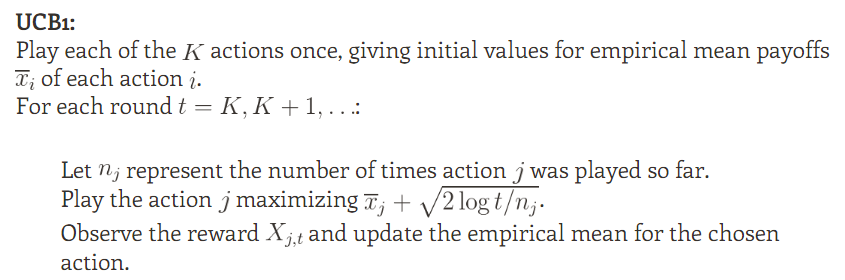

We can see that UCB1’s bound is entirely derived from Hoeffding’s inequality. Besides Hoeffding’s inequality, other inequalities can also derive corresponding bounds. Reinforcement Learning: Exploration vs Exploitation mentions some other inequalities:

Bernstein’s inequality
Empirical Bernstein’s inequality
Chernoff inequality
Azuma’s inequality
…….

UCB2

From the name, you can basically guess that UCB2 is an improvement on UCB1. The improvement is in reducing the upper bound of UCB1’s regret. Regret refers to the gap between the maximum reward obtainable each time and the actually obtained reward. This part involves many mathematical proofs, so I’ll omit it here. For details, refer to Finite-time Analysis of the Multiarmed Bandit Problem. The UCB2 algorithm procedure is shown below, also taken from Finite-time Analysis of the Multiarmed Bandit Problem: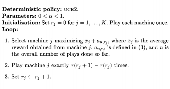

From the flowchart, we can see that UCB2 is similar to UCB1, also calculating a bound for each arm, then selecting an arm based on the arm’s historical reward and bound. However, instead of experimenting once on this arm, we experiment $\tau(r_j+1) - \tau(r_j)$ times. The definitions of $a_{n, r_j}$ and $\tau(r)$ above are as follows. Since $\tau(r)$ must be an integer, we take the ceiling:

\[\begin{align} a_{n,r} = \sqrt{\frac{(1+\alpha)\ln(ne/\tau(r))}{2\tau(r)}} \end{align}\]

\[\begin{align} \tau(r) = \lceil (1+\alpha)^r\rceil \end{align}\]

The $\alpha$ in the above formula is a hyperparameter. According to the experimental results in the paper given above (shown below), this value should not be set too large. The paper’s suggested value is 0.0001: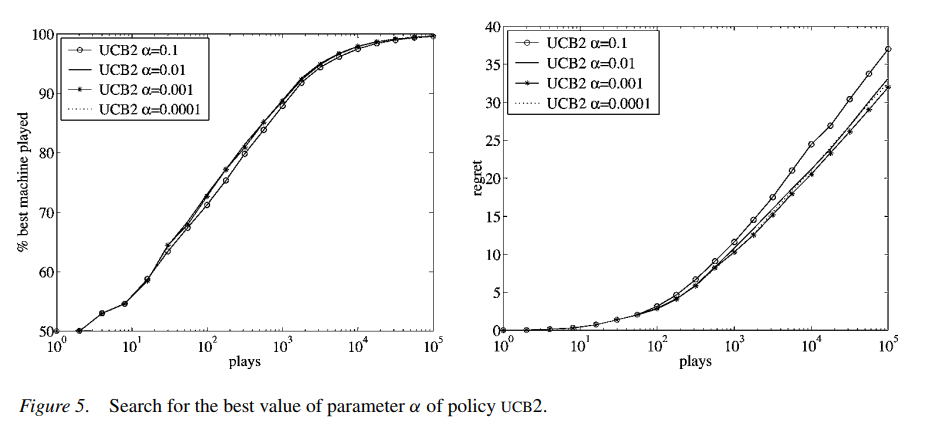

LinUCB

The UCB1 and UCB2 algorithms above both solve the Bernoulli Bandit problem, assuming each arm’s quality follows a Bernoulli distribution. The historically calculated $\overline {x}_j$ (ratio of rewarding experiments to total experiments) is actually the parameter of the Bernoulli distribution.

This statistics-based method is simple but has significant problems, because an arm’s reward is related to multiple factors (for example, an arm may not be rewarding when selected in the morning but is rewarding in the evening). Utilizing this information can make predictions more accurate, but statistics-based methods ignore this.

Different from Bernoulli Bandit, problems utilizing contextual information are the Contextual Bandit problems mentioned above, and LinUCB is designed to solve this problem. In LinUCB, instead of directly defining a probability distribution to describe each arm’s historical reward situation, we assume a linear relationship between the arm’s quality and the feature vector $x$ describing the arm: $x^T \theta$.

This is actually a classic Linear Regression problem (rewards are not limited to 0 and 1). $x$ is a vector composed of the arm’s features (features need to be selected based on the specific problem), and $\theta$ is the model parameter. Each experiment is a sample, with the label being the specific reward.

$\theta$ can be solved from historical samples. When selecting an arm each time, LinUCB uses $x^T \theta$ to replace $\overline {x}_j$ in UCB1 or UCB2, but this is not all of LinUCB. As a UCB-type method, LinUCB still has a bound, because after all, we can only conduct a limited number of experiments on each arm from historical records, and the estimated reward situation still differs from the true one.

The Hoeffding’s inequality used to derive the bound in UCB1 cannot be directly applied to LinUCB. The bound for linear regression was first proposed in the paper Exploring compact reinforcement-learning representations with linear regression. I won’t detail the proof process here. The paper proposing LinUCB A Contextual-Bandit Approach to Personalized News Article Recommendation directly adopted this conclusion, expressed as follows:

\[\begin{align} p(|x_j^T\theta_j - E(r|x_j)| \le \alpha \sqrt{x_j^T(D_j^TD_j+I)^{-1}x_j}) \ge 1- \delta \end{align}\]

This means that for an arm $j$, the difference between the calculated $x_j^T\theta_j$ and the actual expectation being less than $\alpha \sqrt{x_j^T(D_j^TD_j+I)^{-1}x_j}$ has probability greater than $1- \delta$, where $D_j$ is the matrix composed of the features observed for arm $j$ in previous observations. For example, if arm $j$ was observed $m$ times previously, and the feature vector dimension is $d$, then $D_j$ has size $m$ X $d$. $I$ is the identity vector, and $\alpha = 1 + \sqrt{\ln(2/\delta)/2}$. Therefore, as long as $\delta$ is selected based on probability, the bound for each arm can be calculated through $\alpha \sqrt{x_j^T(D_j^TD_j+I)^{-1}x_j}$.

Therefore, the LinUCB algorithm procedure is as follows, including both the arm selection method and the linear regression model update: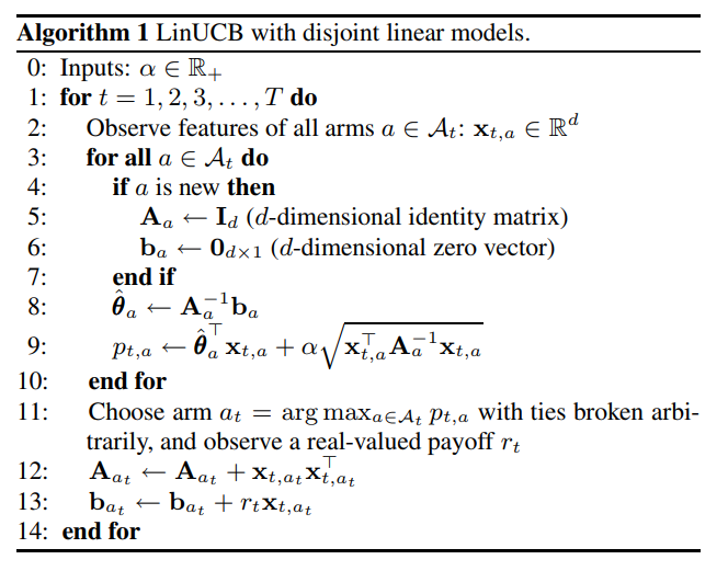

The linear model parameters for each arm above are independent. The paper designed some shared parameters for these models based on this point, replacing the originally calculated $x_j^T\theta_j$ for arm $j$ with $x_j^T\theta_j + z_j^T \beta$, where $\beta$ is the parameter shared by each model, and $z_j^T$ is the feature corresponding to these parameters. For this situation, the paper also has a second algorithm: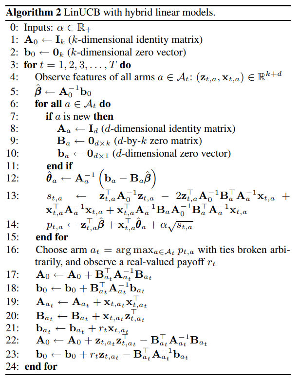

Thompson Sampling Methods

The UCB methods above all adopt the frequentist approach, believing that the metric for judging an arm’s quality is a fixed value. If we had infinite experiments, we could accurately calculate this value. But since only a limited number of experiments can be conducted in reality, the estimated value has bias and needs to be measured by calculating another bound.

The Thompson sampling method introduced below adopts the Bayesian approach, believing that the metric for judging an arm’s quality is not a fixed value but follows some assumed distribution (prior). Through observed historical records, we update the distribution parameters (likelihood) to obtain new distribution parameters (posterior), then repeat this process. When comparison is needed, we randomly generate a sample from the distribution.

Bernoulli Bandit

As mentioned earlier, Bernoulli Bandit assumes that an arm’s quality follows a Bernoulli distribution, meaning whether each experiment obtains a reward follows a Bernoulli distribution with parameter $\theta$:

$p(reward | ) Bernoulli() $

UCB1 and UCB2 in UCB methods both use simple historical statistics to obtain $\overline {x}_j$ to represent $\theta$, but Bayesians believe $\theta$ follows a specific distribution. According to Bayes’ formula:

\[\begin{align} p(\theta|reward) = \frac{p(reward|\theta) p{(\theta)}}{p(reward)} \propto p(reward|\theta) p{(\theta)} ＝Bernoulli(\theta) p(\theta) \end{align}\]

$p(\theta|reward)$ represents the posterior probability updated based on observed experimental reward situations. Since the likelihood $p(reward|\theta)$ is a Bernoulli distribution, to maintain conjugacy for easier calculation, the prior distribution $p(\theta)$ is chosen as a Beta distribution, i.e., $Beta(\alpha, \beta)$. Multiplying the two distributions $Bernoulli(\theta)*Beta(\alpha, \beta)$ yields a new Beta distribution. Simply put:

When $Bernoulli(\theta)$’s result is 1, we get $Beta(\alpha + 1, \beta)$
When $Bernoulli(\theta)$’s result is 0, we get $Beta(\alpha, \beta + 1)$

Therefore, the Thompson Sampling steps for Bernoulli Bandit are as follows, taken from A Tutorial on Thompson Sampling: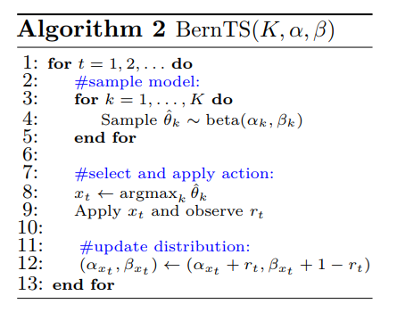

Contextual Bandit

In Bernoulli Bandit, we assume whether an arm obtains a reward follows a Bernoulli distribution, i.e., $p(reward | \theta) \sim Bernoulli(\theta)$.

In Contextual Bandit, we assume the obtained reward has a linear relationship with the feature vector, i.e., $reward = x^T \theta$. Therefore, we cannot directly update $\theta$ through likelihood $p(reward | \theta) \sim Bernoulli(\theta)$ like before.

But following the approach for solving Bernoulli Bandit above, as long as we define $p(reward|\theta)$ and $p(\theta)$ as appropriate conjugate distributions, we can use Thompson Sampling to solve Contextual Bandit, because according to Bayes’ formula:

\[\begin{align} p(\theta|reward) \propto p(reward|\theta) p{(\theta)} \end{align}\]

Theoretically, as long as $p(reward|\theta)$ and $p(\theta)$ are conjugate, it works. But considering the rationality of the assumed distributions, referring to the paper Thompson Sampling for Contextual Bandits with Linear Payoffs, we use normal distributions for both. The paper provides many mathematical proofs, which I’ll omit, and directly give the final conclusion.

For $p(reward|\theta)$, since we estimate reward as $x^T\theta$, we assume the true reward follows a normal distribution centered at $x^T\theta$ with standard deviation $v^2$, i.e., $p(reward|\theta) \sim \mathcal{N}(x^T\theta, v^2)$. The specific meaning of $v$ will be given later.

For computational convenience, $p(\theta)$ generally chooses a form conjugate to $p(reward|\theta)$. Since $p(reward|\theta)$ is a normal distribution, $p(\theta)$ should also be a normal distribution (the conjugate of a normal distribution is still a normal distribution).

To facilitate giving the posterior probability form, the paper first defines the following equations:

\[\begin{align} B(t) = I_d + X^TX \end{align}\]

\[\begin{align} \mu(t) = B(t)^{-1}(\sum_{\tau = 1}^{t-1} x_{\tau}^Tr_{\tau}) \end{align}\]

Here $t$ represents the $t$-th experiment of an arm, $d$ represents the feature dimension, $X$ has the same meaning as introduced in LinUCB, i.e., the matrix composed of this arm’s features from the previous $t-1$ times. In this example, its dimension size is ($t-1$) X $d$. $r_{\tau}$ represents the reward obtained in the $\tau$-th experiment among the previous $t-1$ experiments.

Then $p(\theta)$ at time $t$ follows normal distribution $\mathcal{N}(\mu(t), v^2B(t)^{-1})$, and the posterior probability calculated by multiplying $p(\theta)$ with $p(reward|\theta)$ is $p(\theta|reward) \sim \mathcal{N}(\mu(t+1), v^2B(t+1)^{-1})$.

The $v$ mentioned earlier is defined as $v = R\sqrt{9d\ln(\frac{t}{\delta})}$. Here $t$ and $d$ have the same meanings as above, while $R$ and $\delta$ are two constants that need to be customized, both used in two inequalities to constrain the regret bound, where $R \ge 0$ and $0 \le \delta \lt 1$. The specific equations can be found in the original paper, which I won’t elaborate on.

When $t = 1$, meaning no experiments have been done yet, $p(\theta)$ will be initialized as $\mathcal{N}(0, v^2I_d)$.

The strategy for selecting an arm each time is similar to the Bernoulli Bandit above: each arm’s $p(reward|\theta)$ distribution generates a $\theta$, then we select the arm with the largest $x^t\theta$ for the experiment.

Summary

This article mainly introduced several strategies for the EE problem. Besides the simplest random methods, UCB and Thompson Sampling are two typical methods for this problem. Both methods work by calculating a reward value for each arm, then ranking based on this value and selecting the arm with the largest value.

UCB adopts the frequentist approach, calculating the reward value as historical reward plus a bound. The historical reward can be considered as Exploitation, while the bound is Exploration. In Thompson Sampling, each arm’s reward value is generated from a distribution, without obvious Exploitation and Exploration. However, we can also consider values more likely generated from the distribution as Exploitation, and less likely generated values as Exploration. Additionally, this article focused on the specific procedures of these methods. For more theoretical foundations and mathematical derivations of these methods, refer to the literature below.

References:

开栏：智能决策系列
推荐系统的 EE 问题及 Bandit 算法
Reinforcement Learning: Exploration vs Exploitation
Multi-Armed Bandits and the Gittins Index
Boltzmann Exploration Done Right
Optimism in the Face of Uncertainty: the UCB1 Algorithm
Finite-time Analysis of the Multiarmed Bandit Problem
Exploring compact reinforcement-learning representations with linear regression
A Tutorial on Thompson Sampling
A Contextual-Ba ndit Approach to Personalized News Article Recommendation