Adam is Great, Why Still Miss SGD

Posted on 2019-03-18 标签机器学习 , 数学 , 转载

Haven’t updated in a while. Recently busy writing graduation thesis, just happened to write the optimization-related part, remembered a great article I bookmarked on Zhihu before. Reading it again still feels very beneficial, specially reposting. Original link here, deleted upon infringement.

In the machine learning world, there’s a group of alchemists. Their daily routine is:

Get the ingredients (data), set up the alchemy furnace (model), light the fire (optimization algorithm), then wave the palm-leaf fan waiting for the elixir to come out.

However, anyone who’s been a cook knows: same ingredients, same recipe, but different heat levels produce vastly different flavors. Too little heat leaves it raw, too much burns it, uneven heat makes it half raw half burned.

Machine learning is the same. Model optimization algorithm choice directly relates to final model performance. Sometimes poor results aren’t necessarily feature issues or model design issues, but very likely optimization algorithm issues. (Note: I’ve experienced this personally - once used Adam and immediately fell into local optimum, checked code many times, finally almost despairingly switched to SGD, then results shot up.)

Speaking of optimization algorithms, beginners must start with SGD, while experts will tell you there are better ones like AdaGrad/AdaDelta, or just use Adam mindlessly. But looking at the latest academic papers, you find many experts still using entry-level SGD, at most adding Momentum or Nesterov, and often bashing Adam. For example, a UC Berkeley paper wrote in its Conclusion (Note: this paper is The Marginal Value of Adaptive Gradient Methods in Machine Learning):

Despite the fact that our experimental evidence demonstrates that adaptive methods are not advantageous for machine learning, the Adam algorithm remains incredibly popular. We are not sure exactly as to why ……

Helplessness and bitterness overflow in the words.

Why is this? Could it be that plain and simple is true?

A Framework to Review Optimization Algorithms

First, let’s review various optimization algorithms.

Deep learning optimization algorithms have gone through the development path: SGD -> SGDM -> NAG ->AdaGrad -> AdaDelta -> Adam -> Nadam. Google search reveals many tutorial articles detailing how these algorithms evolved step by step. Here, let’s take a different approach and use a framework to organize all optimization algorithms for a higher-level comparison.

First define: parameters to optimize: \(w\), objective function: \(f(w)\), initial learning rate \(\alpha\)

Then start iterative optimization. In each epoch \(t\), perform the following operations:

Calculate the objective function’s gradient w.r.t. current parameters: \(g_t=\nabla f(w_t)\)
Calculate first-order and second-order moments based on historical gradients: \(m_t = \phi(g_1, g_2, \cdots, g_t)\); \(V_t = \psi(g_1, g_2, \cdots, g_t)\)
Calculate current descent gradient: \(\eta_t = \alpha \cdot m_t / \sqrt{V_t}\)
Update based on descent gradient: \(w_{t+1} = w_t - \eta_t\)

Mastering this framework, you can easily design your own optimization algorithms.

Using this framework, let’s examine the true nature of various mysterious optimization algorithms. Steps 3 and 4 are consistent across algorithms, the main difference lies in 1 and 2.

SGD

First look at SGD. SGD has no concept of momentum, meaning:

\(m_t = g_t\) \(V_t = I^2\)

Substituting into step 3, we can see the descent gradient is the simplest:

\(\eta_t = \alpha \cdot g_t\)

SGD’s biggest disadvantage is slow descent speed, and it may oscillate continuously on both sides of ravines, staying at a local optimum.

SGD with Momentum

To suppress SGD’s oscillation, SGDM thinks the gradient descent process can add inertia. When going downhill, if you find a steep slope, use inertia to go faster. SGDM stands for SGD with momentum, adding first-order momentum on SGD basis:

\(m_t = \beta_1 \cdot m_{t-1} + (1-\beta_1)\cdot g_t\)

First-order momentum is the exponential moving average of gradient directions at various moments, approximately equal to the average of gradient vector sums over the recent \(1/(1-\beta_1)\) moments.

That is, the descent direction at moment t is determined not only by the current point’s gradient direction, but also by the previously accumulated descent direction. \(\beta_1\)’s empirical value is 0.9, which means the descent direction is mainly the previously accumulated descent direction, slightly biased toward the current moment’s descent direction. Imagine a car turning on a highway - while moving forward at high speed with slight bias, sharp turns are dangerous.

SGD with Nesterov Acceleration

SGD has another problem: trapped oscillating in local optimum ravines. Imagine walking into a basin surrounded by slightly higher hills. You feel no downhill direction, so you can only stay there. But if you climb to high ground, you’ll find the outside world is still vast. Therefore, we shouldn’t stay at current position to observe future directions, but take a step forward, look one step ahead, see farther.

NAG stands for Nesterov Accelerated Gradient, an improvement on SGD and SGD-M basis, improving step 1. We know the main descent direction at moment t is determined by accumulated momentum, and current gradient direction doesn’t have much say. So rather than looking at current gradient direction, let’s first see how to walk after following accumulated momentum for one step. Therefore, NAG in step 1 doesn’t calculate current position’s gradient direction, but calculates the descent direction after following accumulated momentum for one step:

\(g_t=\nabla f(w_t-\alpha \cdot m_{t-1} / \sqrt{V_{t-1}})\)

Then combine the next point’s gradient direction with historical accumulated momentum to calculate the current moment’s accumulated momentum in step 2.

AdaGrad

Previously we didn’t use second-order momentum. The appearance of second-order momentum marks the arrival of the “adaptive learning rate” optimization algorithm era. SGD and its variants update each parameter with the same learning rate, but deep neural networks often contain many parameters that aren’t always used (think of large-scale embeddings). For frequently updated parameters, we’ve accumulated much knowledge about them and don’t want individual samples to have too much influence, hoping for slower learning rate; for occasionally updated parameters, we know too little and hope to learn more from each accidentally appearing sample, i.e., larger learning rate.

How to measure historical update frequency? That’s second-order momentum - the sum of squares of all gradient values so far on that dimension:

\(V_t = \sum_{\tau=1}^{t} g_\tau^2\)

Let’s review the descent gradient in step 3:

\(\eta_t = \alpha \cdot m_t / \sqrt{V_t}\)

We can see the actual learning rate changed from \(\alpha\) to \(\alpha / \sqrt{V_t}\). Generally, to avoid zero denominator, a small smoothing term is added. Therefore \(\sqrt{V_t}\) is always greater than 0, and the more frequently a parameter updates, the larger the second-order momentum, the smaller the learning rate.

This method performs very well in sparse data scenarios. But there are also problems: because \(\sqrt{V_t}\) is monotonically increasing, it makes learning rate monotonically decrease to 0, potentially causing training to end prematurely, even if there’s more data later, unable to learn necessary knowledge.

AdaDelta / RMSProp

Since AdaGrad’s monotonically decreasing learning rate change is too aggressive, we consider a strategy to change the second-order momentum calculation method: don’t accumulate all historical gradients, only focus on descent gradients in a past time window. This is the origin of Delta in AdaDelta’s name.

The modification idea is simple. Earlier we said exponential moving average is approximately the average over a past period, so we use this method to calculate second-order accumulated momentum:

\(V_t = \beta_2 * V_{t-1} + (1-\beta_2) g_t^2\)

This avoids the problem of second-order momentum continuously accumulating and causing training to end prematurely.

Adam

Speaking of which, the appearance of Adam and Nadam is very natural - they are the culmination of previous methods. We saw SGD-M adds first-order momentum on SGD basis, AdaGrad and AdaDelta add second-order momentum on SGD basis. Using both first-order and second-order momentum is Adam - Adaptive + Momentum.

SGD’s first-order momentum:

\(m_t = \beta_1 \cdot m_{t-1} + (1-\beta_1)\cdot g_t\)

Plus AdaDelta’s second-order momentum:

\(V_t = \beta_2 * V_{t-1} + (1-\beta_2) g_t^2\)

The two most common hyperparameters in optimization algorithms \(\beta_1\), \(\beta_2\) are here, the former controls first-order momentum, the latter controls second-order momentum.

Nadam

Finally Nadam. We said Adam is the culmination, but it surprisingly missed Nesterov - how can this be tolerated? Must add it. Following NAG’s step 1:

\(g_t=\nabla f(w_t-\alpha \cdot m_{t-1} / \sqrt{V_t})\)

This is Nesterov + Adam = Nadam.

Speaking of which, you can probably understand why people often say Adam/Nadam are currently the most mainstream and easy-to-use optimization algorithms. Newbies can try them first - fast convergence and great results.

So why does Adam keep getting bashed and despised by academia? Is it just for paper padding?

Adam’s Two Crimes

From a theoretical perspective, each generation is more perfect, Adam/Nadam has reached perfection, so why do people still not forget SGD?

For example. Many years ago, photography was very distant from ordinary people. Ten years ago, point-and-shoot cameras became popular, tourists almost had one each. After smartphones appeared, photography entered thousands of households - just point and shoot with your phone, front and back 20 million pixels, illuminating your beauty (wait, what is this mess). But professional photographers still like DSLRs, tirelessly adjusting aperture, shutter, ISO, white balance… a bunch of terms selfie enthusiasts never care about. Technological progress makes simple operations produce good results, but in specific scenarios, to shoot the best results, still need deep understanding of light, structure, equipment.

Optimization algorithms are similar. In the previous article, we used the same framework to categorize various algorithms. We can see everyone reaches the same goal through different paths, just adding various active learning rate controls on SGD basis. If you don’t want fine tuning, Adam is obviously easiest to start with directly.

But such simple operations don’t necessarily fit all situations. If researchers can deeply understand data, they can more freely control various optimization iteration parameters, achieving better results isn’t strange. After all, if carefully tuned parameters still can’t beat simple Adam, it’s undoubtedly challenging top researchers’ alchemy experience!

Adam’s First Crime: May Not Converge

This is from On the Convergence of Adam and Beyond in anonymous review for ICLR 2018, one of the top deep learning conferences, discussing Adam algorithm’s convergence, proving through counterexample that Adam may not converge in some cases. (Note: This paper became ICLR 2018 Best Paper)

Recall the learning rates of various optimization algorithms mentioned above:

\(\eta_t = \alpha / \sqrt{V_t}\)

Here, SGD doesn’t use second-order momentum, so learning rate is constant (in practice, learning rate decay strategy is used, so learning rate decreases). AdaGrad’s second-order momentum continuously accumulates and monotonically increases, so learning rate monotonically decreases. Therefore, both types of algorithms make learning rate continuously decrease, eventually converging to 0, and the model also converges.

But AdaDelta and Adam are different. Second-order momentum is accumulation within a fixed time window. As the time window changes, encountered data may change drastically, making \(V_t\) sometimes large sometimes small, not monotonic. This may cause learning rate oscillation in late training, leading to model unable to converge.

This paper also gives a correction method. Since Adam’s learning rate is mainly controlled by second-order momentum, to ensure algorithm convergence, we can control second-order momentum changes to avoid up and down fluctuation.

\(V_t = max(\beta_2 * V_{t-1} + (1-\beta_2) g_t^2, V_{t-1})\)

With this modification, we guarantee \(||V_t|| \geq ||V_{t-1}||\), thus making learning rate monotonically decreasing.

Adam’s Second Crime: May Miss Global Optimum

Deep neural networks often contain many parameters. In such extremely high-dimensional space, non-convex objective functions have many ups and downs, with countless highlands and lowlands. Some are peaks that momentum can easily overcome; but some are plateaus that may take many explorations to exit, so training stops.

Two recent Arxiv papers discuss this problem.

The first is the previously mentioned paper that bashes Adam hardest: The Marginal Value of Adaptive Gradient Methods in Machine Learning. It says for the same optimization problem, different optimization algorithms may find different answers, but adaptive learning rate algorithms often find very poor answers. Through a specific data example, they show that adaptive learning rate algorithms may overfit early-appearing features, and later-appearing features are hard to correct early fitting effects.

Another paper is Improving Generalization Performance by Switching from Adam to SGD, conducting experimental verification. They tested on CIFAR-10 dataset, Adam converges faster than SGD, but final convergence result isn’t as good as SGD. They further found mainly because Adam’s learning rate is too low in late stages, affecting effective convergence. They tried controlling Adam’s learning rate lower bound and found much better results.

So they proposed a method to improve Adam: Use Adam early, enjoying Adam’s fast convergence advantage; later switch to SGD, slowly finding the optimal solution. This method has been used by researchers before, but mainly choosing switch timing and post-switch learning rate based on experience. This paper automates this switching process, giving methods for choosing SGD switch timing and calculating learning rate, with results looking good too.

Should I Use Adam or SGD?

So, having talked so much, is Adam better or SGD better? This may be hard to say in one sentence. Looking at various papers in academic conferences, many use SGD, quite a few use Adam, and many prefer AdaGrad or AdaDelta. Researchers probably try each algorithm once and use whichever gives better results.

From these papers bashing Adam, most construct some extreme examples to demonstrate the possibility of Adam failing. These examples are generally too extreme and may not happen in practice, but this reminds us of the necessity of understanding data for algorithm design. The evolution history of optimization algorithms is based on optimizing under some assumption about data, so whether an algorithm is effective depends on whether your data fits the algorithm’s appetite.

Algorithms are beautiful, but data is fundamental.

On the other hand, while Adam and similar have simplified parameter tuning, they haven’t once and for all solved the problem. Default parameters are good, but not universally applicable. Therefore, on the foundation of fully understanding data, still need sufficient parameter tuning experiments based on data characteristics and algorithm characteristics to find your own optimal alchemy solution. At this point, whether Adam or SGD doesn’t matter to you.

Young man, practice alchemy well.

Optimization Algorithm Selection and Usage Strategies

In the previous two sections, we used a framework to organize various optimization algorithms and pointed out potential problems with adaptive learning rate optimization algorithms represented by Adam. So how should we choose in practice? This article introduces Adam+SGD combination strategy and some useful tricks.

Core Differences Between Different Optimization Algorithms

From the framework in the first article, we see the most core difference between different optimization algorithms is the descent direction in step 3:

\(\eta_t = (\alpha/ \sqrt{V_t} ) \cdot m_t\)

In this formula, the first part is actual learning rate (i.e., descent step size), the second part is actual descent direction. SGD algorithm’s descent direction is the reverse of that position’s gradient direction, SGD with first-order momentum’s descent direction is that position’s first-order momentum direction. Adaptive learning rate optimization algorithms set different learning rates for each parameter, setting different step sizes in different dimensions, so their descent direction is scaled first-order momentum direction.

Different descent directions may cause different algorithms to reach completely different local optima. An empirical analysis of the optimization of deep network loss surfaces did an interesting experiment. They mapped objective function values and corresponding parameters’ hyperplane to 3D space, so we can intuitively see how each algorithm finds the lowest point on the hyperplane.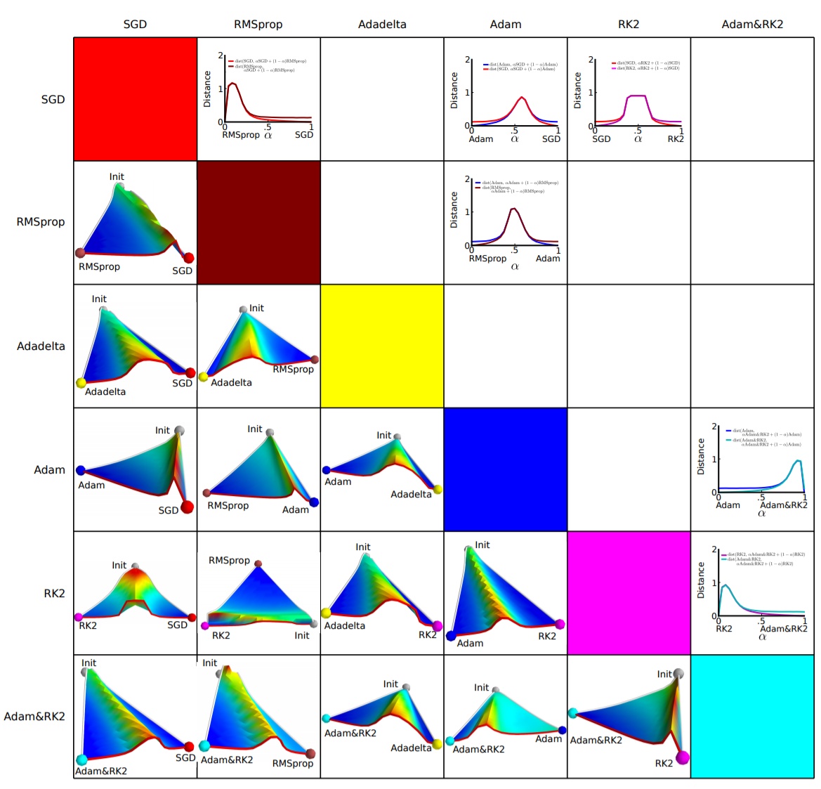

The above figure shows the paper’s experimental results. Horizontal and vertical coordinates represent the dimensionally reduced feature space, region color represents objective function value changes, red is plateau, blue is lowland. They did paired experiments, letting two algorithms start from the same initialization position, then compare optimization results. We can see, almost any two algorithms walk to different lowlands, often separated by a very high plateau. This shows different algorithms choose different descent directions at plateaus.

Adam+SGD Combination Strategy

It’s the choice at every crossroad that determines your destination. If heaven could give me one more chance, I would say to that girl: SGD!

The pros and cons of different optimization algorithms remain a controversial topic with no conclusion. Based on feedback I’ve seen in papers and various communities, the mainstream view is: Adam and other adaptive learning rate algorithms have advantages for sparse data and converge very fast; but carefully tuned SGD (+Momentum) often achieves better final results.

So we might think, can we combine these two, first use Adam for fast descent, then use SGD for fine tuning, getting the best of both worlds? Simple idea, but there are two technical issues:

When to switch optimization algorithm? - If switching too late, Adam may have already run into its own basin, no matter how good SGD is it can’t get out.
What learning rate to use after switching algorithm? - Adam uses adaptive learning rate, depending on second-order momentum accumulation. If SGD continues training, what learning rate to use?

The paper mentioned in the previous article, Improving Generalization Performance by Switching from Adam to SGD, proposes solutions to these two problems.

First look at the second question, what learning rate to use after switching. Adam’s descent direction is:

\(\eta_t^{Adam} = (\alpha/ \sqrt{V_t} ) \cdot m_t\)

And SGD’s descent direction is:

\(\eta_t^{SGD} = \alpha^{SGD} \cdot g_t\)

\(\eta_t^{SGD}\) can definitely be decomposed into the sum of two directions: one in \(\eta_t^{Adam}\)’s direction and one orthogonal to it, as shown below, where p is Adam descent direction, g is gradient direction, r is SGD learning rate.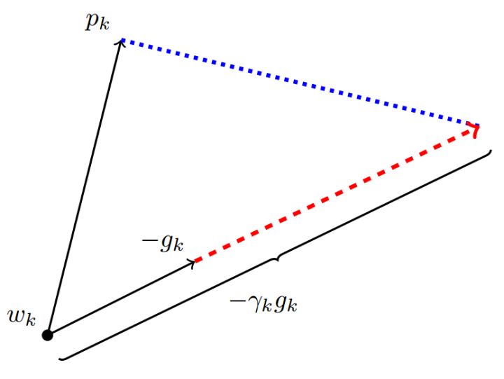

Its projection on \(\eta_t^{Adam}\) direction means the distance SGD moves forward in the descent direction determined by Adam algorithm, and the projection on \(\eta_t^{Adam}\)’s orthogonal direction is the distance SGD moves forward in its own chosen correction direction.

If SGD is to walk the unfinished path of Adam, it must first take over Adam’s banner - take one step along \(\eta_t^{Adam}\) direction, then take a corresponding step along the orthogonal direction.

Thus we know how to determine SGD’s step size (learning rate) - SGD’s orthogonal projection on Adam descent direction should exactly equal Adam’s descent direction (including step size). That is:

\(proj_{\eta_t^{SGD}} = \eta_t^{Adam}\)

Solving this equation, we get the learning rate for continuing with SGD:

\(\alpha_t^{SGD} = ((\eta_t^{Adam})^T\eta_t^{Adam})/((\eta_t^{Adam})^Tg_t)\)

To reduce noise impact, the author uses moving average to correct learning rate estimation:

\(\lambda_t^{SGD} = \beta_2 \cdot \lambda_{t-1}^{SGD}+(1-\beta_2) \cdot \alpha_t^{SGD}\)

\(\tilde{\lambda}_t^{SGD}=\lambda_t^{SGD}/(1-\beta_2^t)\)

Here directly reuses Adam’s \(\beta_2\) parameter.

Now look at the first question, when to switch algorithms.

The author’s answer is also simple: when SGD’s corresponding learning rate moving average is basically unchanged, i.e.:

\(|\tilde{\lambda}_t^{SGD} - \alpha_t^{SGD}|<\epsilon\). After each iteration, calculate SGD successor’s corresponding learning rate. If it’s basically stable, then SGD takes over with \(\tilde{\lambda}_t^{SGD}\) as learning rate.

Common Tricks for Optimization Algorithms

Finally, sharing some tricks in optimization algorithm selection and usage.

First, there’s no conclusion on which algorithm is better. If just starting out, prioritize SGD+Nesterov Momentum or Adam. (Standford 231n: The two recommended updates to use are either SGD+Nesterov Momentum or Adam)
Choose algorithms you’re familiar with - so you can more skillfully use your experience for parameter tuning
Fully understand your data - if data is very sparse, prioritize adaptive learning rate algorithms.
Choose based on your needs - in model design experiments, to quickly verify new model effects, can first use Adam for fast experimental optimization; before model deployment or result publication, can use carefully tuned SGD for model extreme optimization.
Use small dataset for experiments first. Paper Stochastic Gradient Descent Tricks points out, SGD convergence speed has little relation to dataset size. Therefore can first use a representative small dataset for experiments, test best optimization algorithm, and find optimal training parameters through parameter search.
Consider combining different algorithms. First use Adam for fast descent, then switch to SGD for sufficient fine tuning. Switching strategy can refer to the method introduced in this article.
Dataset must be fully shuffled. This way when using adaptive learning rate algorithms, can avoid certain features appearing concentrated, causing sometimes over-learning, sometimes under-learning, making descent direction deviate.
During training, continuously monitor objective function values and metrics like accuracy or AUC on training and validation data. Monitoring training data ensures model is sufficiently trained - correct descent direction and high enough learning rate; monitoring validation data avoids overfitting.
Formulate an appropriate learning rate decay strategy. Can use periodic decay strategy, like decay once every certain epochs; or use performance metrics like accuracy or AUC for monitoring, when test set metric doesn’t change or decreases, reduce learning rate.