Reading Notes on "Real-time Personalization using Embeddings for Search Ranking at Airbnb"

Real-time Personalization using Embeddings for Search Ranking at Airbnb is KDD 2018’s best paper. Reading through it, at first glance it seems to just apply word2vec to generate user and item embeddings. But reading more carefully, there are many details worth examining. This style is similar to YouTube’s 2016 paper Deep Neural Networks for YouTube Recommendations. Both are very practical papers worth reading. The two articles represent two major approaches for generating embeddings in deep learning: unsupervised and supervised. This article mainly describes Airbnb’s approach and key details.

Airbnb’s work addresses the business need: when users search on the rental app, a list of recommendation results needs to be returned. The paper mentions Airbnb uses mainstream Learning To Rank technology. For LTR technical details, see Microsoft’s From RankNet to LambdaRank to LambdaMART: An Overview. Airbnb uses pairwise mode LambdaRank. This paper mainly describes how to generate user and item embeddings through word2vec as features for the ranking model (the paper also calls items listings, so these terms have the same meaning).

This article’s main highlights:

1. Incorporating positive feedback (user final booking as global context) and negative feedback (host rejection as additional dataset) signals into skip-gram training 2. When doing negative sampling, considering specific business not just sampling from full set 3. Same uid samples are sparse, so user embedding granularity changes from uid to user type, avoiding insufficient embedding learning due to sparse samples

These 3 points are improvements the authors made considering specific business scenarios, which I think is what makes this paper most worth learning: don’t blindly apply algorithms, but make appropriate adaptations and improvements based on current specific business.

Offline Training

Offline training in the paper is divided into two parts: short-term interest and long-term interest.

For short-term interest, 800 billion click sessions are used to train listing embeddings.

For long-term interest, 50 million users’ booked listings are used to train user type embeddings and listing type embeddings.

The training method is basically word2vec’s skip-gram. Below describes both parts’ specific training details.

Listing Embedding

In short-term interest, only item embeddings are generated. Training samples are click sessions (analogous to a sentence in NLP), defined in the paper as a series of user click events. When building this training dataset, the key is how to define session length. In the paper, when two clicks are more than 30 minutes apart, they belong to different sessions.

Assuming total training set is \(S\), each session is \(s=(l_1,l_2...l_M) \in S\), then through word2vec’s skip-gram we can write the loss:

\[\begin{align} L=\sum_{s \in S}\sum_{l_i \in s}(\sum_{-m \le j \le m,j \ne 0}^M \log p(l_{i+j}|l_i))\tag{1} \end{align}\]

Here \(m\) is a hyperparameter representing skip-gram training window size. The probability can be expressed through embedding vectors and softmax:

\[\begin{align} p(l_{i+j}|l_i) = \frac{\exp(v_{l_j}^T v_{l_{i+j}}^{'})}{\sum_{l=1}^{|V|}\exp(v_{l_i}^Tv_{l}^{'})}\tag{2} \end{align}\]

Where \(|V|\) is all items set, \(v\) and \(v'\) represent input vector and output vector respectively. They’re actually the same item’s representations in two parameter matrices in skip-gram model, i.e., parameter matrices W and W’ shown below. See CS224n: Natural Language Processing with Deep Learning.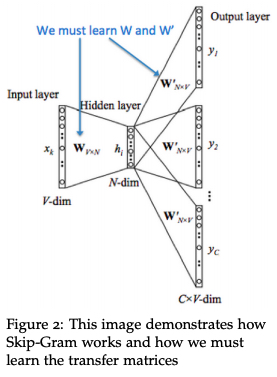

Similar to word2vec, since this set is generally very large, computing probability formula (2) takes very long due to denominator summation. To accelerate training, word2vec proposes negative sampling strategy. Simply, for each clicked item in a session, select positive pairs \((l, c)\) from window \(m\) as positive set (denoted \(D_p\)), while randomly selecting negative pairs \((l, c)\) from entire item set \(|V|\) as negative set (denoted \(D_n\)). Instead of softmax, use sigmoid to write the solution:

\[\begin{align} \arg\max_{\theta} \sum_{(l,c) \in D_p} \log\frac{1}{1+e^{-v_{c}^{'}v_l}} + \sum_{(l,c) \in D_n} \log\frac{1}{1+e^{v_{c}^{'}v_l}} \tag{3} \end{align}\]

The parameter \(\theta\) to solve is each item’s embedding \(v_l\). This is basically the original word2vec skip-gram algorithm. The following points are the authors’ modifications to word2vec based on business, very worth learning.

(1) Using supervision signal as global context

In Airbnb’s business, sessions can actually be divided into two types: sessions with final booking and sessions without booking. The paper calls them booked sessions and exploratory sessions. Both are supervision signals. The paper only uses the first supervision signal. Then formula (3) becomes:

\[\begin{align} \arg\max_{\theta} \sum_{(l,c) \in D_p} \log\frac{1}{1+e^{-v_{c}^{'}v_l}} + \sum_{(l,c) \in D_n} \log\frac{1}{1+e^{v_{c}^{'}v_l}} + \\\ \log \frac{1}{1+e^{-v_{l_b}v_l}}\tag{4}\end{align}\]

In formula (4), \(v_{l_b}\) is the embedding of booked item \(l_b\). The figure below more intuitively shows how this supervision signal works. We can see each central listing/item updates together with booked listing/item to compute probability once, so this listing is called global context. Its effect is strengthening the relationship between all items clicked before purchase and the final booked item.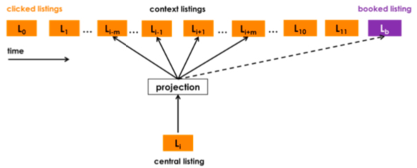

(2) Controlling negative sampling space

As mentioned above, negative sampling randomly selects \(n\) items from full set as negatives. But in Airbnb’s business, a user usually only books in one market (travel destination). The negative sampling results in \(D_p\) candidates all from same market, while \(D_n\) candidates often aren’t from same market. The paper calls this imbalanced not optimal. I guess the reason is during prediction, candidate items are basically from same market, while random \(D_n\) makes same-market positive-negative items less distinguishable. Therefore, in addition to original negative sampling, add \(D_{m_n}\) randomly selecting negatives from same market. The final loss form:

\[\begin{align} \arg\max_{\theta} \sum_{(l,c) \in D_p} \log\frac{1}{1+e^{-v_{c}^{'}v_l}} + \sum_{(l,c) \in D_p} \log\frac{1}{1+e^{v_{c}^{'}v_l}} + \\\ \log \frac{1}{1+e^{-v_{l_b}v_l}}+\sum_{(l,m_n) \in D_{m_n}} \log\frac{1}{1+e^{v_{m_n}^{'}v_l}}\tag{5} \end{align}\]

(3) Cold start item embedding

In recommendation systems, many new items are added daily, and some items have no click sessions at all, can’t train corresponding embeddings through word2vec. For these cold start items, the paper uses a common and effective approach: select \(k\) most similar items with embeddings based on cold start item’s attributes, then do mean pooling. Selection method uses item meta-data like price, listing type, etc.

user_type/listing_type embeddings

The training method above only uses click sessions and only generates listing embeddings. The paper considers this short-term interest, reflected in the session partition rule mentioned above - two clicks more than 30 min apart are different sessions. Under this partition, captured is user’s short-term interest, and all items in one session are basically from same market.

To (1) capture user’s longer-cycle interest (2) capture cross-market listing embedding relationships, the paper trains user embedding + listing embedding through skip-gram. Compared to only training listing embedding for short-term interest, the paper calls this long-term interest.

The training data above is 800 billion click sessions, while capturing long-term interest training uses 50 million users’ booked listings.

Assuming total training set is \(S_b\), each booked listing is \(s_b=(l_{b1},l_{b2}...l_{bM}) \in S\), representing all listings booked by a user (sorted by time).

Compared to rich click sessions above, this problem is more severe:

1. Data is sparser - above is click events, here is conversion events
2. Some users’ booked listing length might only be 1, can’t directly train with skip-gram
3. For each entity to learn embedding sufficiently, each entity should appear at least 5-10 times, but many listings are booked fewer than 5 times

Problems 2 and 3 are actually manifestations of problem 1. So the paper’s solution to these three problems is converting id to type, essentially converting id features to more generalized features. Basic conversion method maps user/listing based on meta info to a type, then uses this type to replace user/listing id. Mapping table: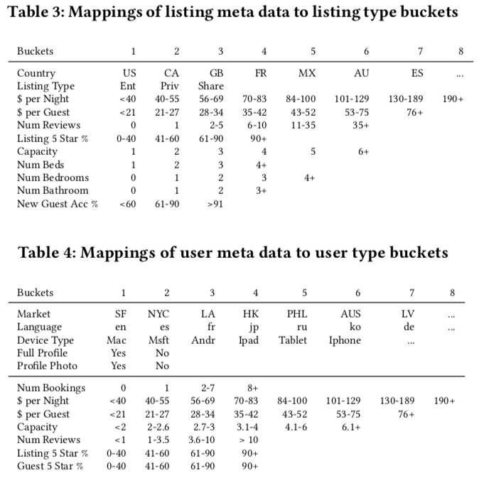

After solving sparse data problem, remaining issue is how to train user_type embedding and listing_type embedding in same vector space through word2vec? Because original word2vec sequences are usually same-attribute items.

The paper’s solution is straightforward: transform each user’s booked listing \(s_b=(l_{b1},l_{b2}...l_{bM}) \in S\) to \(s_b=(u_{type1},l_{type1}...u_{typeM}, l_{typeM}) \in S\). Note although each session’s sequence represents same user_id, user_type changes over time, but paper doesn’t mention time window for changing user_type. Guess is change whenever it changes, then insert into booked listing’s corresponding time position (there’s an issue - this seems unable to solve booked listing length 1 data).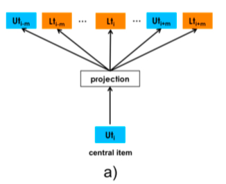

After negative sampling, loss is same as formula 3. Below is central item as user type case (listing type similar):

\[\begin{align} \arg\max_{\theta} \sum_{(u_t,c) \in D_{book}} \log\frac{1}{1+e^{-v_{c}^{'}v_{u_t}}} + \sum_{(u_t,c) \in D_{neg}} \log\frac{1}{1+e^{v_{c}^{'}v_{u_t}}} \tag{6} \end{align}\]

Compared to extra negative sampling for same-market items when training listing embeddings above, here it’s not done because booked sessions’ items already include different markets, so no extra processing needed.

Additionally, Airbnb’s business context also has host feedback data, i.e., some users book but hosts reject (possible reasons like incomplete user info, low rating, etc.). This negative feedback is beneficial for user_type embedding learning. For these negative feedback signals, Airbnb adds them as follows:

For each central item, training data besides \(D_{book}\) and \(D_{neg}\) from negative sampling, also defines \(D_{rej}\) containing pairs \((u_t, l_t)\) where user was rejected. When central item is user (listing similar), loss:

\[\begin{align} \arg\max_{\theta} \sum_{(u_t,c) \in D_{book}} \log\frac{1}{1+e^{-v_{c}^{'}v_{u_t}}} + \sum_{(u_t,c) \in D_{neg}} \log\frac{1}{1+e^{v_{c}^{'}v_{u_t}}} + \\\ \sum_{(u_t,l_t) \in D_{neg}} \log\frac{1}{1+e^{v_{l_t}v_{u_t}}} \tag{7}\end{align}\]

The skip-gram after adding this supervision signal: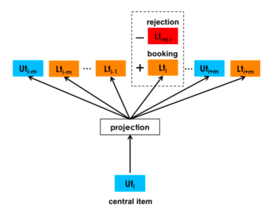

Training Details

Above describes general training process, but some training details are also important, especially for work with specific business context. The paper only describes training listing embedding details.

Training data details:

• As mentioned, used 800 million click sessions. Partition criterion is two consecutive clicks by same user more than 30min apart are different sessions.
• Removed invalid clicks (defined as page stay time less than 30s)
• 5x upsampling for booked sessions

Training details:

• Daily update, using sliding window from current time backward for several months of training data
• Retrain listing embedding daily (random initialization), not finetuning on previously trained embeddings. Paper says this works better than finetuning.
• Embedding dimension 32 (trade-off between effectiveness and resources), skip-gram window 5, 10 iterations works best.

Notably, the reason daily retraining listing embedding works is Airbnb doesn’t directly use embedding as model input feature, but uses embedding-calculated similarity as input feature. If using user/listing embedding directly as feature in samples, daily retraining would likely not work. Analysis:

Because user/item similarity computed from embedding is determined by user/item’s relative position in training dataset, this information doesn’t change much in daily training data. But each retraining with random initialization easily leads to same training set producing embeddings in different vector spaces twice. If embedding is directly used as NN model feature, same user/item might have very different vectors yesterday vs today, which is obviously unreasonable for a feature.

Embedding Validity Verification

After training embeddings, how to judge validity is worth discussing, especially with deep learning lacking interpretability. The paper uses several methods worth learning:

1. Visualization
2. Compute cosine similarity between listing embeddings
3. Re-rank historical log items based on embedding similarity, check booked item position (smaller is better)

Method (1) is visualization, also common for evaluating embedding validity. Typical approach is clustering then examining item correlation in each cluster. For listing embeddings trained above, k-means into 100 clusters. Since each Airbnb item corresponds to a geographic point, the paper does two types of visualization. First, coloring different cluster points differently on map:

Paper says clustering results are also good for redefining each travel market’s scope.

Second visualization is for specific listing embedding, selecting k-nearest listing embeddings and visually examining similarity of corresponding properties:

Method (2) computes embedding cosine similarity. In two tables below, partition listing embeddings by item meta info, then compute mean cosine similarity between item embeddings in each partition and other item embeddings. Results show items with more similar price and property type have higher listing embedding cosine similarity, so this information can be learned into listing embeddings.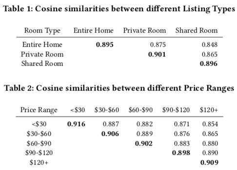

Method (3) is an embedding quality evaluation method designed by paper based on business. Motivation: use embedding info to re-rank historical search sessions, compare with search rank model’s historical ranking.

Basic approach: select all historical search sessions where user’s booked item appeared, each session contains other candidate items. Based on user’s clicked items’ embeddings, compute each candidate item embedding’s similarity with these clicked item embeddings, re-rank by similarity, observe booked item’s rank (smaller is better).

Since these are historical sessions, candidate items were already ranked by Airbnb’s search rank, serving as baseline. Paper selects each user’s last 17 clicks to compute similarity. Results: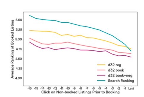

Meanings in figure above:

• search ranking: Posterior ranking, i.e., actual historical session ranking
• d32: Embedding trained by formula (3), i.e., original word2vec method
• d32 book: Embedding trained by formula (4), i.e., adding booked item as global context
• d32 book+neg: Embedding trained by formula (5), i.e., negative sampling specifically considering same-market negatives

Figure shows d32 book+neg performs best.

Online Serving

How to use trained embeddings in serving? Paper mainly uses two places:

1. Search Ranking: User search ranking model
2. Similar Listing Recommendation: Similar items dynamic recommendation on item page

Search Ranking

For NN models, embedding can be directly input as feature. But Airbnb’s ranking model isn’t NN, but tree-based LambdaRank. Model details won’t be expanded here - see paper’s Section 4.4.

Using tree models means embedding can’t be directly input, need to construct continuous features. Below mainly describes how these features are constructed and online results.

The paper mainly uses similarity computed between embeddings as continuous features. Feature list: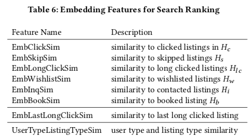

Symbol meanings in figure:

• \(H_c\): Listing ids user clicked in past two weeks
• \(H_{lc}\): Listing ids user clicked and stayed more than 60s
• \(H_s\): Other listing ids skipped when user clicked a listing (e.g., clicked 4th ranked, skipped first 3)
• \(H_w\): Listing ids user added to wishlist in past two weeks
• \(H_i\): Listing ids user contacted but didn’t book in past two weeks
• \(H_b\): Listing ids user booked in past two weeks

So first 6 features represent candidate’s similarity with items user historically interacted with. Besides, paper also partitions features by market. For \(H_c\), partition into \(H_c(market1)\), \(H_c(market2)\)…, then mean-pool all listing embeddings in same market, called market-level embedding. Then compute candidate listing’s similarity with each market-level embedding and take maximum. For candidate \(l_c\), first feature calculation:

\[\begin{align} EmbClickSim(l_c, H_c) = \max_{m \in M} cos(v_{l_i}, \sum_{l_h \in m, l_h \in H_c}v_{l_h}) \end{align}\]

I have a question: why take max instead of adding all features? Because this approach essentially crosses market and similarity features. Adding all would expand original feature count. Paper doesn’t explain this - perhaps many crossed features are empty?

The two features after the table above compute similarly, just not partitioned by market because unlike listings, these don’t have clear market concept. EmbLastLongClickSim captures user’s recent interest, UserTypeListingTypeSim captures user’s longer-term generalized interest.

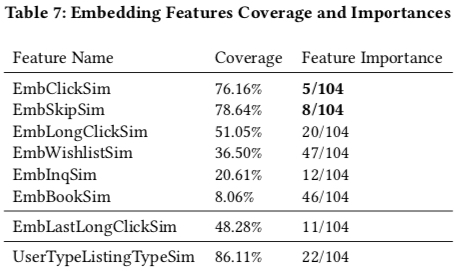
The above features are accumulated for 30 days. Below is feature coverage and importance (from tree model training results). Airbnb’s model has 104 features. 5 embedding-constructed features are in top 20 important features. Notable points:

• EmbClickSum is most important among embedding-constructed features, reflecting user’s short-term interest
• For booking features, user long-term interest is better than short-term interest (UserTypeListingTypeSim importance higher than EmbBookSim). Another possible reason is EmbBookSim data is sparser - a user typically books once in two weeks.

Additionally, “Real-time” in title is reflected in Table 6’s features changing in real-time with user behavior.

Similar Listing Recommendation

This recommends similar items on each listing detail page, mainly using listing embeddings’ cosine similarity to select top-k most similar items. Paper compares current Airbnb similar item recommendation strategy with this embedding-based method. Online AB experiment shows this method improves CTR about 21% and CVR about 4.9% vs current method.

Summary

I think this paper covers three aspects:

1. How to train and generate embeddings
2. How to evaluate trained embedding validity
3. How to use embeddings online

Training method uses word2vec’s skip-gram. Training data uses user click sessions and book sessions, with business-specific modifications to skip-gram like market-level negative sampling, booked listing as global context, rejected orders as negatives, etc. For sparse conversion data, converting id embedding to type embedding alleviates the issue of insufficient embedding learning with sparse data. Training details are also worth referencing.

For evaluating embedding validity, besides common visualization, paper uses two other worth-learning methods: first, after determining certain dimensions, compare listing embedding similarity across dimensions; second, re-rank historical ranking results based on listing embedding similarity while observing final booked listing’s position in re-ranked results.

For online use of embeddings, since Airbnb uses tree models, can’t directly input embeddings as features. Paper computes embedding similarities as continuous features for model input.

Finally, Zhihu discussion How to evaluate Airbnb’s Real-time Personalization winning KDD 2018 best paper? has many interpretations worth reading. Recommend this answer.