Reading Notes on "Bid Optimization by Multivariable Control in Display Advertising"

Recommendation and advertising are two important businesses for many internet companies. Recommendation aims for DAU growth, or traffic growth, while advertising uses this traffic for monetization. Both problems are similar - each time traffic arrives, selecting top-k candidates from a large candidate set, both using the retrieval + ranking architecture, possibly with coarse ranking in between. Essentially, this is a trade-off between effectiveness and engineering.

If I had to identify the biggest technical difference between the two, I think it’s bidding. In advertising scenarios, the advertiser role is introduced, so besides user experience, we need to satisfy the advertisers’ needs (like volume, cost, etc.) to bring sustained revenue growth. Advertisers express their needs most directly through bidding, meaning how much they’re willing to pay per click/convert (truthful telling). This leads to the bidding research area. Many related papers are collected in rtb-papers.

This article mainly discusses Alibaba’s 2019 KDD paper Bid Optimization by Multivariable Control in Display Advertising. This paper solves two core bidding problems: bid formula and price adjustment strategy. From derivation of optimal bid formula to construction of bid controller, the paper’s overall modeling approach is worth learning. The entire derivation paradigm can be extended to more general bidding scenarios with strong practicality. I recommend reading the original paper.

Bidding can be considered to consist of two main parts technically: bid formula and controller. For example, the common CPC bid formula is bid * ctr, and the most common controller is PID. The bid formula is easy to understand, but why do we need a controller to adjust prices instead of bidding according to the advertiser’s given bid? I think there are two main reasons:

1. To satisfy various advertiser needs: For example, when uniform delivery is needed (spending budget evenly throughout the day), a controller is needed to control spending curve trend to match overall traffic curve trend. When cost needs to be maintained, a controller is needed to lower prices when cost is high and raise prices when cost is low. When volume is needed while allowing slight cost increase, bidding can be more aggressive when cost is controllable.

2. CTR/CVR estimation isn’t completely accurate: Common CTR/CVR overestimation easily leads to cost overrun because the calculated ecpm = bid×ctr×cvr is also overestimated. The fundamental reason is there’s no absolute ground truth in CTR/CVR estimation - we get click/conversion or not, but need to estimate click/conversion probability.

As mentioned, the paper mainly covers two parts: optimal bid formula derivation and controller. The following content will describe both aspects.

Optimal Bid Formula

The paper’s scenario is maximizing advertiser’s total value across all auctions while maintaining click cost and budget. The optimization problem can be written as: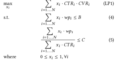

Symbol meanings:

• \(N\): Total auction opportunities for the ad plan
• \(x_i\): Probability of winning the i-th auction
• \(wp_i\): Winning price for the i-th auction, i.e., bid price must be ≥ this value to win
• \(B\): Total budget for the plan
• \(C\): Set click cost

Notably, we don’t need to directly solve this optimization problem, but only need to derive the solution form when optimal, then use it as the optimal bid formula. In other words, we don’t care about the specific optimal value of \(x_i\), but rather what form other variables should take when \(x_i\)’s solution is optimal.

Paper’s Original Derivation

The paper converts the primal problem to a dual problem through duality theory in optimization, as shown below. For detailed duality theory, refer to the Duality Theory section in Optimization Course Summary or the Duality Theory lecture notes.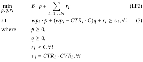

In the above figure, \(p\), \(q\), and \(r\) are variables in the dual problem, corresponding to three constraints in the primal problem: budget, cost, and range constraint on \(x\). According to Complementary Slackness theorem, we get the following two equations. Detailed Complementary Slackness description also refers to the above links.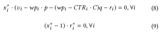

In the above formulas, \(x_i^{*}\) and \(r_i^{*}\) represent optimal solutions for primal and dual problems respectively. Symbols with * superscript indicate optimal solutions. So far, all formulas are derived based on optimization theory. But the next step is a bit of a leap - the paper directly sets the optimal bid formula as:

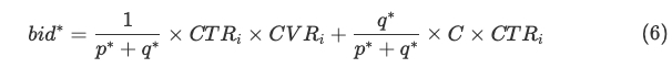
Then the value \(v_i\) brought to the advertiser in those formulas can be written as \(v_{i} = bid_{i} - wp_{i}\). Substituting formula (6) into this equation, then substituting \(v_i\) into formula (8) in the figure above, we get formula (10) and its classification discussion results: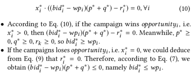

The two classification results above actually indicate that whether the optimal solution \(x^*\) wins the auction (\(x=1\)) or loses (\(x=0\)), bidding according to formula (6) always guarantees the solution is optimal.

Another Derivation Approach

I said the final derivation is a bit of a leap because how was the optimal bid formula in formula (6) given? It seems unlikely to be randomly guessed. The paper doesn’t describe this in detail. Here I attempt to provide another solution approach using Lagrangian duality. For this content, refer to the Lagrangian duality section in Convex Optimization Summary.

For the primal problem in LP1 above, we can write its augmented Lagrangian function as (temporarily ignoring \(x\)’s range constraint):

\[\begin{align} L(x,p,q) = \sum_{i=1\dots N}-x_iCTR_iCVR_i + p(\sum_{i=1\dots N}x_iwp_i-B) + q(\sum_{i=1\dots N}x_i(wp_i-CTR_iC)) \end{align}\]

Where \(p>=0, q>=0\), so the primal problem can be written as:

\[\begin{align} \max_{p, q}\min_{x_i}L(x,p,q) \end{align}\]

If we need to solve this problem, we’d need to convert to Lagrangian dual problem and solve through SMO or similar algorithms. But we don’t need the exact solution, just the optimal solution’s expression. So we can let \(\frac{\partial{L(x,p,q)}}{\partial{x}}=0\), solving to get:

\[\begin{align} wp_i = \frac{1}{p+q} × CTR_{i} × CVR_{i} + \frac{q}{p+q} × C × CTR_{i} \end{align}\]

We can see the derived form of winning price \(wp_i\) is the same as the optimal bid formula in formula (6)!!!

However, there are still issues with the above derivation. We solved for optimal \(wp_i\), but the bid variable doesn’t explicitly appear in the augmented Lagrangian function. We can approximately consider them equal. Second, \(x_i\)’s own constraint (range 0~1) isn’t explicitly considered in the augmented Lagrangian function. My understanding is when solving optimization problems, we can ignore certain conditions, then do classification discussion after solving. This part is actually what the original paper does after deriving formula (10).

Summary

Combining both derivations above, we get the optimal bid formula as shown in formula (6). The formula’s \(p\) and \(q\) are two hyperparameters, variables to be solved in the dual problem. If we need to solve them, it means getting all posterior data from auctions, but in practice we need to give bid at auction time, which becomes a chicken-and-egg problem. Later we’ll describe how to solve this through a controller. The idea is not directly solving the original optimization problem but gradually approaching the optimal solution through approximation.

Returning to formula (6)’s optimal bid formula, if we write it as c_bid * ctr form, we get: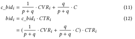

More intuitively drawn as below. From the figure, even when CVR is 0, bid isn’t necessarily 0. This differs from common ecpm = bid×ctr×cvr, meaning some low-CVR but high-CTR traffic can still be acquired. Also, c_bid line passes through two fixed points: (-qC, 0) and (pC, C). These points’ specific meanings will be described in detail in the controller section.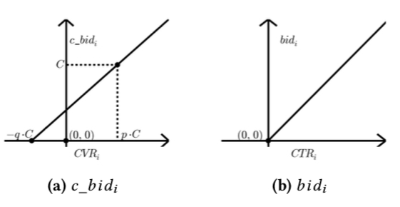

Price Adjustment Strategy

As mentioned, solving for optimal values of \(p\) and \(q\) in the optimal bid formula requires posterior data after auctions, but bid needs to be given at auction time. This creates a chicken-and-egg problem. A straightforward idea: can we use historical data to find optimal \(p\) and \(q\), then apply to next time period’s bidding? The paper mentions this, and the answer is no. This approach assumes auction traffic distribution is basically unchanged, but the bidding environment is dynamically changing due to multiple factors (including auction traffic, CTR, CVR, etc.), meaning historical optimal won’t be future optimal. In practice, my experience confirms this.

Since the bidding environment changes in real-time, dynamic price adjustment is needed. In adjustment strategy, we first need to clarify two points: control objective and control variable. Taking the classic PID controller as example, as shown below, control objective is making \(r(t)\) and \(y(t)\) as close as possible, control variable is \(x(t)\).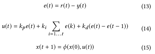

Each variable adjustment requires calculating current error through formula (13), then calculating control signal \(u(t)\) through formula (14) (where \(k_p\), \(k_i\), \(k_d\) are three predetermined hyperparameters), finally using \(u(t)\) through adjustment formula (actuator model) \(\phi(x(0), u(t))\) to get the final adjusted value.

PID is a commonly used and effective method for single-variable control, but our problem above is a multi-variable control problem, where control variables are \(p\) and \(q\), control objectives are controlling budget spend and maintaining click cost. For this problem, an intuitive approach is using dual PID for independent control, but these control variables are often not independent, so dual PID isn’t optimal, as will be detailed later.

Parameter Analysis

First, let’s analyze which control objectives are affected by control variables \(p\) and \(q\).

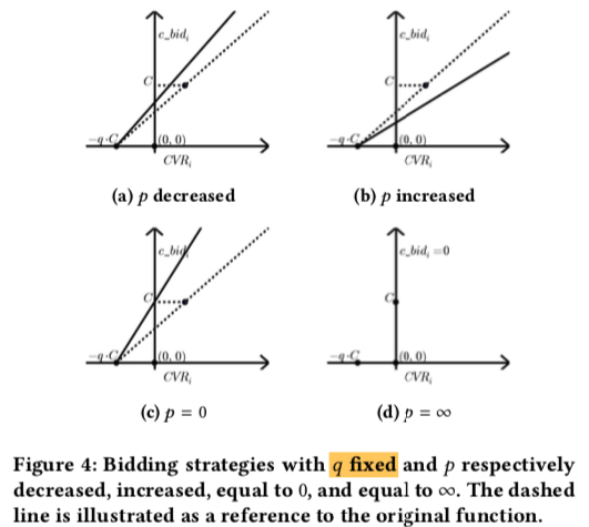
As shown in Figure 4 below, when fixing \(q\) and changing \(p\), the change in c_bid is shown, with dashed line showing bid before change, solid line after change. From the figure:

• Bid line always passes through point (-qC, 0)
• As \(p\) decreases, bid line’s slope increases, indicating higher bid, and more budget consumed. As \(p\) increases, the opposite effect occurs.
• When \(p\) takes minimum value of 0, there’s no budget constraint. Bid formula degenerates to \(C×CTR+\frac{1}{q}CTR×CVR\). The first term can be considered click-only bidding to maintain click cost \(C\), the second term is for achieving \(\max v=CTR×CVR\) objective.

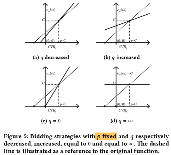
Similarly, Figure 5 shows c_bid changes when fixing \(p\) and changing \(q\). From the figure:

• Bid line always passes through point (pC, C)
• As \(q\) decreases, bid line’s slope increases, indicating higher bid for traffic with CVR higher than pC, lower bid for CVR lower than pC. As \(q\) increases, the opposite effect occurs.
• When \(q\) takes minimum value of 0, there’s no click cost constraint. Bid formula degenerates to \(\frac{1}{p}CTR×CVR\), where symbol \(C\) representing bid cost doesn’t appear, meaning achieving \(\max v=CTR×CVR\) objective while controlling budget through \(q\).

Controller

From the above analysis, parameter \(p\) is used to control budget usage, while parameter \(q\) controls click cost. This is consistent with the constraint conditions when deriving optimal bid formula above.

Therefore, a simple strategy is using two independent PIDs to separately control variables \(p\) and \(q\), with control objectives being budget and click cost, as shown below.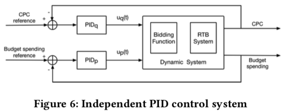

But as mentioned earlier, these two aren’t completely independent. For example, raising or lowering prices to maintain click cost also affects budget usage, and vice versa. Therefore, two completely independent PIDs aren’t the optimal choice - control should consider mutual influence between variables.

Model Predict Control (MPC) has research on such problems, but the paper doesn’t directly adopt this method because it considers “modeling the highly non-linear RTB environment is costly and even impractical”. Instead, it uses a linear model for fitting. I think this is feasible because adjustment is often divided into multiple time slices, with control in each time slice. Using linear fitting in each time slice, as long as time slices are sufficiently small, the overall result can theoretically fit nonlinear curves.

The main modeling idea is directly modeling the relationship between variables \(p\), \(q\) and objectives cost, CPC through two linear regression models (i.e., modeling the bidding environment with respect to cost and CPC in the original paper). The specific approach: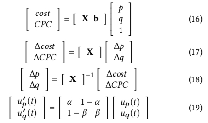

In formula (16) above, \(X\) and \(b\) are 2×2 matrix and 2×1 matrix respectively. If expanded, they’re actually two linear regression models.

Furthermore, formula (17) indicates that given control objectives \(\Delta cost\) and \(\Delta CPC\) (adjustment is done in time slices; before each adjustment, we can calculate required \(\Delta cost\) and \(\Delta CPC\) for current time slice based on current accumulated spend and cost posterior data), we can achieve the objectives by adjusting \(p\) and \(q\) by \(\Delta p\) and \(\Delta q\) respectively. I have a question here: why can \(b\) be eliminated?

Although the paper doesn’t explicitly mention it, I think by formula (17) we could already do adjustment, just differently from the paper’s approach. Here’s a brief description. First we need to obtain \(X\) in formula (17), whose parameters can be obtained from training data. The training dataset is (\(\Delta p\), \(\Delta q\), \(\Delta cost\), \(\Delta CPC\)) from several time slices before current time, then \(X\) can be obtained through conventional training. This way, during each time slice adjustment, with pre-calculated \(X\) and next time slice’s control objectives \(\Delta cost\), \(\Delta CPC\), we can find optimal \(\Delta q\) and \(\Delta p\) through grid search.

Formula (18) is obtained by multiplying both sides of formula (17) by inverse of matrix \(X\). Formula (19) is the paper’s adjustment approach: first, the PID adjustment formula (14) can convert \(\Delta cost\) and \(\Delta CPC\) in formula (18) to \(u_{p}(t)\) and \(u_{q}(t)\). Meanwhile, only two variables \(\alpha\) and \(\beta\) are used to approximate the inverse of matrix \(X\) (theoretically should have 4), and it’s considered that \(p\), \(q\)’s control signals \(u'_{p}(t)\), \(u'_{q}(t)\) are linear combinations of \(u_{p}(t)\), \(u_{q}(t)\). The paper states this makes the controller more robust and stable against the changing environment. The paper says \(\alpha\) and \(\beta\) are obtained from training set (see experimental results section below).

Therefore, according to formula (19), the overall control system becomes: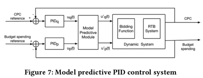

Experimental Setup and Evaluation

Basic Setup

The paper doesn’t conduct online experiments but evaluates through offline methods.

The dataset is 40 Taobao plans with 20M bid logs total. Each bid log’s key information is \(wp_i\), \(CTR\), \(CVR\). Training and test sets are divided by time.

Evaluation metrics mainly include two:

• \(CPC_{ratio}\): Proportion of plans maintaining click cost
• \(Value_{ratio}\): Ratio of value obtained by each plan when re-delivering with optimal bid formula to its theoretical optimal (\(\le 1\))

Implementation Details

Besides, when calculating control signal through PID, the paper weights the error, while traditional PID gives equal weight to all errors. The weighting method is shown in formula (21), and \(u_{q}(t)\) calculation mentioned earlier is shown in formula (22).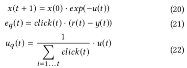

Besides error weighting, formula (20) is also interesting. Each time adjusting target value \(x\) through control signal, it’s not based on last value \(x(t)\), but initial value \(x(0)\).

Additionally, adjustment frequency is once per hour. Hyperparameters in PID (\(k_p\), \(k_i\), \(k_d\)) and \(\alpha\), \(\beta\) in formula (19) are all found through grid search on training set.

Therefore, overall experimental steps:

1. Calculate optimal \(p\), \(q\) based on training dataset as initial values
2. Simulate bidding on test dataset using optimal bid formula and adjustment strategy
3. Terminate when plan budget is exhausted or all logs are replayed

Results Comparison

Experimental results shown below. Figure 8 shows budget consumption, Figure 9 shows cost situation. Left figures show real-time metrics, right figures show cumulative metrics. From the figures, budget consumption fits well in both real-time and cumulative, while click cost has fluctuations in real-time but cumulative cost is relatively stable.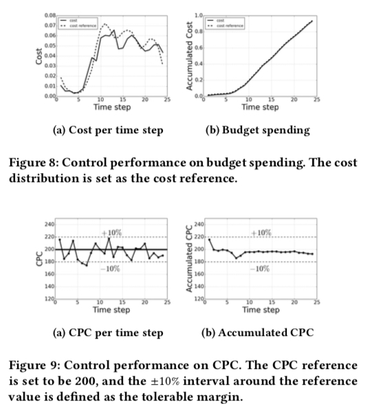

Besides, the paper compares with several other methods. Results shown below, where I-PID and M-PID are methods proposed in this paper, indicating PID independence or not. Results show using the paper’s bid formula with adjustment strategy considering control variable relationships performs best, confirming that two completely independent PIDs aren’t optimal - control should consider mutual influence between variables.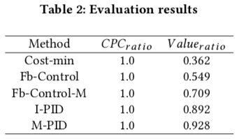

Summary

In summary, this paper first models the method to be solved as an optimization problem, then derives the optimal solution’s form through duality theory rather than the solution itself. Then it describes an adjustment strategy in multi-variable control system that considers relationships between control variables, with experimental results proving this strategy outperforms two independent PIDs. The shortcoming is no online experiments - after all, offline experiment environment is basically fixed, and re-bidding won’t change the environment, unlike online changes being so dramatic. But the paper’s overall modeling approach is worth learning and can serve as a paradigm for more general bidding scenarios.