Delayed FeedBack In Computational Advertising
Conversion has delay, meaning users may convert some time after clicking, and often the deeper the conversion funnel, the longer the delay. In computational advertising, delayed feedback mainly affects the following two scenarios:
- CVR model training
- Posterior-based bidding strategy adjustment
For scenario 1, the impact is: (1) sending samples to the model too early treats events that will eventually convert but haven’t received labels yet as negative examples, causing model underestimation; (2) sending samples to the model too late, i.e., waiting a sufficiently long time for all samples before sending to the model, causes the model to not update timely.
For scenario 2, the impact is when the controller controls cost/value=target, the denominator will be smaller than the actual value, causing control instability.
This article mainly introduces three papers’ approaches to this problem in scenario 1. Some methods involved can also be applied to scenario 2 (and if problem 1 can be well solved, bidding can also be based on predictions rather than posterior data).
The first paper is an earlier proposed solution, introducing a latent variable to assist modeling, while separately modeling delay time. The overall modeling approach is worth learning.
The second paper extends the first paper. The first paper models the callback delay time with exponential distribution, while this paper borrows KDE (Kernel density estimation) to learn arbitrary distributions for modeling callback delay time.
The third paper compares several methods’ effects on offline data and online experiments, with changes mainly in the loss function. It includes the first paper’s method and others using positive-unlabeled learning/importance sampling to derive new losses.
Modeling Delayed Feedback in Display Advertising(2014)
This paper is from Criteo in 2014, modeling delayed feedback. The modeling approach is worth learning. For this paper, refer to a previously written article:
《Modeling Delayed Feedback in Display Advertising》 阅读笔记
A Nonparametric Delayed Feedback Model for Conversion Rate Prediction(2018)
This paper improves the callback delay function on the first paper’s basis. The first paper used exponential distribution to model callback delay, here KDE (Kernel density estimation) ideas are used to replace the first paper’s exponential distribution with arbitrary distribution, which is the meaning of nonparametric in the paper name.
Basic symbol definitions are similar to the first paper: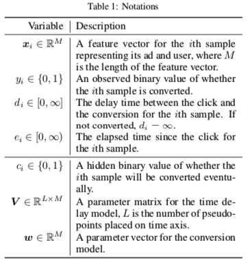
The paper mainly derives through Survival analysis. Simply speaking, survival analysis mainly studies the following field:
Survival analysis is a branch of statistics for analyzing the expected duration of time until one or more events happen, such as death in biological organisms and failure in mechanical systems.
Survival analysis concepts and derivations used in the paper: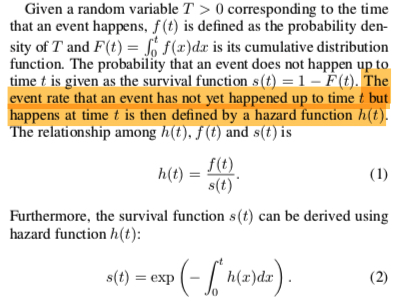
The first paper also uses the above derivation. \(f(t)\) is exponential distribution’s pdf, \(s(t)\) is exponential distribution’s cdf, and \(h(t)\) is \(\lambda(x)\) in the first paper.
From the above expression, the key to solving \(s(t)\) is finding hazard function \(h(x)\). Hazard function’s meaning is the event rate for first event occurrence at current moment. Compared to the first paper directly setting \(h(x) = \lambda(x) = w\_dx\), here borrowing Kernel density estimation ideas, the hazard function is written as follows (\(L\) is a hyperparameter, representing \(L\) pseudo-points on the time axis):
\[\begin{align} h(d_i; x_i, V) = \sum_{l=1}^{L}\alpha_l(x_i;V)k(t_l, d_i) \end{align}\]
The figure below more intuitively describes how this form fits arbitrary distributions: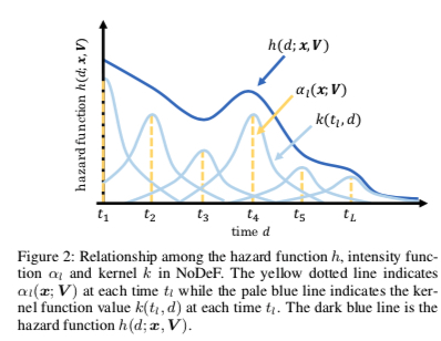
Above \(\alpha_l, k\) are defined as follows. Intuitively, \(\alpha_l\) represents the current pseudo-point’s contribution to the overall hazard function, \(k(t_l, \tau)\) means training samples closer to current pseudo-point \(t_l\) have greater influence on current pseudo-point \(t_l\)’s parameter \(V_l\) (imagine gradients of each \(V_l\) during backprop):
\[\begin{align} \alpha_l(x_i; V) = (1+\exp(-V_{l}^{T}x_i))^{-1} \end{align}\]
\[\begin{align} k(t_l, \tau) = \exp(-\frac{(t_l-\tau)^2}{2h^2}) \end{align}\]
After writing the hazard function, from formula (2):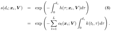
Then paper1’s callback delay probability can be written as:
\[\begin{align} p(d_i|x_i, c_i = 1) = s(d_i; x_i, V )h(d_i; x_i, V) \end{align}\]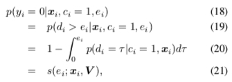
The training algorithm is the same EM algorithm as paper1: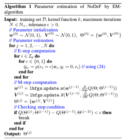
The above form borrows KDE ideas. KDE can be understood as a method to write pdf of arbitrary distributions. For derivation of this part, here’s an intuitive answer: 什么是核密度估计?如何感性认识?
Addressing Delayed Feedback for Continuous Training with Neural Networks in CTR prediction(2019)
This is a paper from Twitter, mainly comparing several methods’ effects on the delayed feedback problem.
Faked negative weighted
The delayed feedback problem can also be understood from another angle: the observed sample distribution is biased distribution \(b\), but we need to solve for the expectation of true sample distribution \(p\). Importance sampling is a method to solve this problem. Wikipedia’s brief introduction:
In statistics, importance sampling is a general technique for estimating properties of a particular distribution, while only having samples generated from a different distribution than the distribution of interest
A more 通俗 explanation on Zhihu: 重要性采样(Importance Sampling. The paper can write the true distribution’s expectation as:
\[\begin{align} E_p[\log f_{\theta}(y|x)] = E_b[\frac{p(x,y)}{b(x,y)} f_{\theta}(y|x)] \end{align}\]
That is, weighting samples by \(w(x,y) = \frac{p(x,y)}{b(x,y)}\) on observed biased distribution \(b\). Then the loss function can be written as: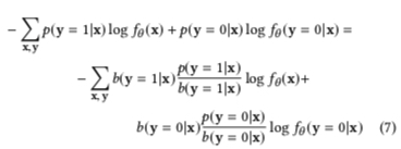
This method treats all samples as negative samples initially, then passes one more positive sample when positive sample is called back. Assuming \(N\) is all samples, \(M\) is positive samples among them:
\[\begin{align} b(y=1|x) = \frac{M}{M+N} = \frac{\frac{M}{N}}{1+\frac{M}{N}} = \frac{p(y=1|x)}{1+p(y=1|x)} \end{align}\]
\[\begin{align} b(y=0|x) = 1- b(y=1|x)= \frac{1}{1+p(y=1|x)} \end{align}\]
That is, formula (7) above can be written as formula (10) below. Positive samples in distribution \(b\) need weight \(1+p(y=1|x)\), negative samples need weight \(p(y=0|x)(1+p(y=1|x))\):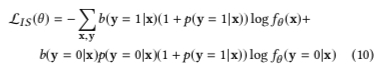
But here \(p\) is unknown, so the paper uses model prediction \(f_{\theta}\) to approximate.
Additionally, importance sampling is also applied in reinforcement learning’s off-policy strategy. Simply speaking, it optimizes target strategy \(\pi\)’s value function through sequence distribution generated by behavior strategy \(b\). For difference between on-policy and off-policy, refer to this answer: 强化学习中 on-policy 与 off-policy 有什么区别?)
Fake negative calibration
This method directly lets the model learn biased distribution \(b\), then inversely derives \(p(y=1|x)\) probability based on formulas derived in Faked negative weighted above. From:
\[\begin{align} b(y=1|x) = \frac{M}{M+N} = \frac{\frac{M}{N}}{1+\frac{M}{N}} = \frac{p(y=1|x)}{1+p(y=1|x)} \end{align}\]
We can derive:
\[\begin{align} p(y=1|x) = \frac{b(y=1|x)}{1-b(y=1|x)} \end{align}\]
This method can be considered a post calibration. Besides this, there’s also a method that corrects during training, called prior correction. The basic idea is to add a transformation layer to the predicted logit during training. Simple derivation follows:
Assuming under true distribution, positive sample count is \(P\), negative sample count is \(N\).
Then serving output probability should be:
\[\begin{align} \frac{P}{P+N} = \frac{1}{1+e^{-x}} \end{align}\]
But during training, due to the above mechanism, each sample appears once as negative sample. Also assuming negative sample sampling with rate \(r\):
\[\begin{align} \frac{P}{r*(P+N)+P} = \frac{1}{1+e^{-x^{*}}} \end{align}\]
Through transformation:
\[\begin{align} \frac{P}{r*(P+N)+P} = \frac{P/(P+N)}{r+P/(P+N)} = \frac{1/(1+e^{-x})}{r + 1/(1+e^{-x})} \end{align}\]
Letting:
\[\begin{align} \frac{1/(1+e^{-x})}{r + 1/(1+e^{-x})}=\frac{1}{1+e^{-x^{*}}} \end{align}\]
We can derive:
\[\begin{align} x^{*} = -(\ln r+ \ln(1+e^{-x})) \end{align}\]
That is, when calculating logit during training, use \(\frac{1}{1+e^{-x^{*}}}\) instead of \(\frac{1}{1+e^{-x}}\).
Positive-Unlabeled Learning
The paper has almost no derivation here. Detailed derivation can refer to Learning Classifiers from Only Positive and Unlabeled Data. Basic idea is quite similar to the first paper. Won’t elaborate, mainly quoting some key derivation steps:
A key assumption about the training data is that they are drawn randomly from \(p(x,y,s)\), and for each tuple \(< x,y,s >\) that is drawn, only \(< x,s >\) is recorded. Here \(s\) is the observed label and \(y\) is the actual label, which might not have occurred yet. Along with this, it is assumed that labeled positive examples are chosen completely randomly from all positive examples, i.e. \(p(s = 1|x, y = 1) = p(s = 1|y = 1)\)
Based on above assumption: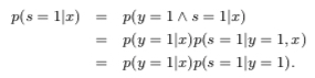
The value of the constant \(c = p(s = 1|y = 1)\) can be estimated using a trained classifier \(g\) and a validation set of examples. Let \(V\) be such a validation set that is drawn from the overall distribution \(p(x, y, s)\) in the same manner as the nontraditional training set. Let \(P\) be the subset of examples in \(V\) that are labeled (and hence positive). The estimator of \(p(s = 1|y = 1)\) is the average value of \(g(x)\) for \(x\) in \(P\). That is \(\frac{1}{n}\sum_{x \in P}g(x)\)
For solving, all samples’ expectation/likelihood can be written as: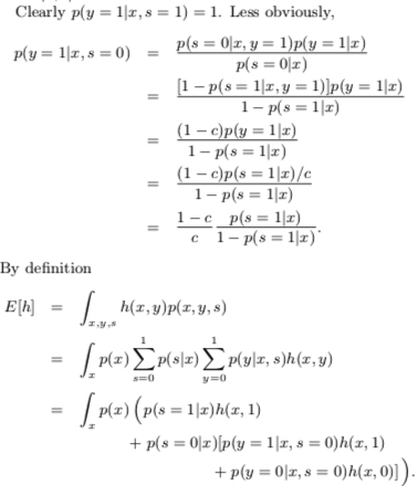
Then the final loss function form is: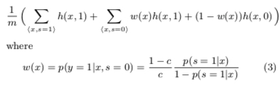
Summary
This article mainly introduced several methods to solve the delay feedback problem. The first paper introduced a latent variable and separately modeled conversion delay and conversion. The modeling approach is worth learning. The second paper improved the first paper’s conversion delay model. The third paper introduced several methods that treat all samples as negative samples initially and input to the model again when positive samples are called back, but this causes training and serving inconsistency (inconsistent positive/negative sample ratio). The paper also proposed several solutions.