Exposure Bias In Machine Learning
Machine learning essentially learns the data distribution. Its effectiveness assumes that training and serving data are Independent and Identically Distributed (IID). However, in practice, due to biased sampling and specific scenario constraints, training samples and serving samples are not IID. In advertising scenarios, the most typical example is CVR model training, where training samples are all post-click, but during serving, the CVR model faces all retrieved samples. This type of problem is called exposure bias or sample selection bias. Besides exposure bias, position bias is also a common bias.
This article first briefly introduces common biases in machine learning, then focuses on exposure bias (also called sample selection bias) and current solution approaches. The author summarizes them into three main categories: Data Augmentation, IPS, and Domain Adaptation.
Bias In Recommender System
Besides the exposure bias that this article focuses on, the survey Bias and Debias in Recommender System: A Survey and Future Directions describes several biases in current recommender systems. The paper divides the recommender system into three main modules: User, Data, and Model, and summarizes 7 types of bias arising from interactions between modules as shown below: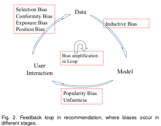
- User->Data: The process of generating training data, also the main source of Bias
- Position Bias (implicit): Users tend to interact with items in higher positions
- Exposure/Observation Bias (implicit): Labeled data is all exposed; unexposed data cannot determine its label
- Selection Bias (explicit): Users tend to rate items they like or dislike (an important cause of exposure bias; many papers treat this as exposure bias)
- Conformity Bias (explicit): Users’ ratings tend to align with group opinions
- Data->Model: The process of training models using data
- Inductive Bias: Refers to assumptions the model makes for generalization, such as Occam’s razor, SVM’s assumption of linear separability, etc. This bias doesn’t bring explicit defects
- Model->User Interaction: The process of model prediction
- Popularity Bias: The long-tail effect, where popular items get higher exposure probability because the model tends to recommend them (caused by unbalanced training data)
- Unfairness: Some predictions have gender or racial discrimination (caused by unbalanced training data)
The causes, effects, and solutions for each bias above can be summarized in the following table: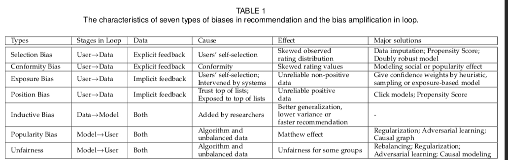
As we can see, these biases are not isolated but interact and worsen each other. Position bias and exposure bias are among the most common and well-studied areas. Below we detail methods for addressing exposure bias. Note that selection bias faces the same problem as exposure bias, so methods here also apply; bias-related methods can refer to the paper above.
Solutions to Exposure Bias
Exposure bias, also known as Sample Selection Bias (SSB), is essentially a training-serving inconsistency problem. This problem often arises from specific business scenario constraints, where training data samples are only a small portion of serving data, because other samples weren’t exposed/clicked and thus couldn’t get their labels.
As mentioned at the beginning, for CVR models, samples that weren’t clicked cannot determine whether they converted; similarly, for CTR models, samples without exposure opportunities cannot determine whether they would be clicked. But during serving, CTR/CVR models face all samples, many of which were never exposed, causing training-serving inconsistency.
Current solutions to this problem include the following approaches (not limited to the survey paper above):
- Data Augmentation: The most naive idea is to utilize samples that didn’t enter the training set as much as possible. Much research gives unobserved/unclicked samples a relatively accurate label. This includes three main methods:
- The crudest is treating all unexposed samples as negative samples, then giving them different weights based on different strategies
- Training an imputation model to predict labels for unexposed samples
- Modeling through multitask learning, using all samples from the previous conversion target (ESMM)
IPS (Inverse Propensity Score): This method assumes sample exposure or click follows a Bernoulli distribution, then derives from probability theory: as long as each exposed sample is weighted (weight being the inverse propensity score), the expectation calculated on exposed samples equals the expectation on all samples. This is essentially importance sampling.
Domain Adaptation: Similar to transfer learning, treating exposed/clicked samples as source domain and all samples as target domain, using domain adaptation methods for debiasing.
Data Augmentation
As mentioned above, the most naive idea is to utilize unobserved samples. This includes three main methods: all negative with confidence, imputation model, and multitask learning.
all negative with confidence
The first method treats all unobserved samples as negative. The core is how to give each sample a reasonable confidence, which is essentially sample weighting. The survey above introduces three methods: Heuristic, Sampling, Exposure-based model.
Heuristic attempts to use user activity level, user preference, item popularity, user-item feature similarity as confidence for (user, item) pairs. The idea is that higher user activity, more popular items, and higher user-item matching mean higher sample confidence. However, this method often lacks feasibility because the actual confidence values are hard to obtain, their scale is difficult, and generating confidence for large datasets is challenging.
Sampling: TODO
Exposure-based model: TODO
imputation model
The second method is intuitive: train an imputation model to label unexposed/unclicked samples, then train the model based on these imputed labels. The imputation model can be trained separately or jointly with the target model. The drawback is obvious: generated imputed labels lack absolute ground truth for evaluation. This is actually a drawback of all methods that directly generate labels for samples.
multitask learning
The third method uses multitask learning. The main idea is simultaneously modeling the current task and its shallower task, thereby indirectly utilizing unexposed/unclicked data. The well-known approach is Alibaba’s 2018 ESMM paper: Entire Space Multi-Task Model: An Effective Approach for Estimating Post-Click Conversion Rate. This paper addresses bias in CVR models due to missing unclicked samples by adding two auxiliary tasks (CTR and CTCVR). The overall model structure is shown below: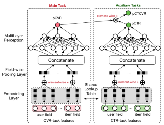
The loss function is (\(y\) represents click event, \(z\) represents conversion event):
\[\begin{align} L(\theta_{ctr},\theta_{cvr}) &= \sum_{i=1}^{N}l(y_i,f(x_i;\theta_{ctr})) \notag \\\ &+\sum_{i=1}^{N}l(y_i\& z_i,f(x_i;\theta_{ctr})×f(x_i;\theta_{cvr})) \notag \end{align}\]
We can consider the model utilizes samples as (show, click, convert) pairs. Compared to traditional CVR models, ESMM can utilize exposed but unclicked samples (the last column in the table below, 0/1 indicates whether the corresponding intermediate event occurred):
| show | click | convert |
|---|---|---|
| 1 | 1 | 1 |
| 1 | 1 | 0 |
| 1 | 0 | 0 |
During prediction, the following conditional probability formula ensures the CVR value is unbiased statistically:
\[\begin{align} p(z=1|y=1,x) = \frac{p(y=1,z=1|x)}{p(y=1|x)} \end{align}\]
Experimental results are shown below. Method meanings: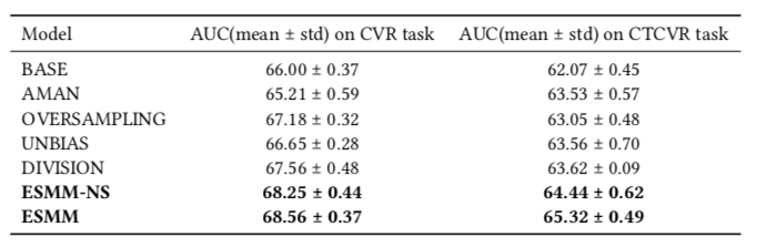
- BASE: Standard CVR model
- AMAN: Negative sampling for negative samples
- OVERSAMPLING: Oversampling positive samples
- UNBIAS: Using pCTR as rejection probability as in this paper
- DIVISION: Modeling pCTR and pCTCVR separately, then calculating pCVR using the formula above
- ESMM-NS: ESMM without shared bottom
- ESMM: ESMM with shared bottom
IPS (Inverse Propensity Score)
Inverse Propensity Score estimates a propensity score for each labeled sample, intuitively meaning the probability of the sample entering the training set (being labeled). For CTR models, propensity is the exposure probability; for CVR models, propensity is the click probability.
IPS actually borrows from Importance Sampling, weighting each sample by a probability value, statistically proving that the expectation calculated from observed data equals the expectation from all data. The derivation can be simply described as follows:
Let \(L\) be the number of samples with observed labels, and \(L'\) include all samples including unobserved ones (\(L' \gg L\)). The unbiased optimization objective should be (\(y_i\) and \(p_i\) represent label and prediction):
\[\begin{align} \min \sum_{i=1}^{L'} l(y_i, p_i) \tag{1} \end{align}\]
Now let \(O_i \in \lbrace 0, 1 \rbrace\) indicate whether the \(i\)-th sample was observed. Assume \(O_i\) follows a Bernoulli distribution \(O_i \sim Bern(z_i)\), where \(z_i\) is the probability of sample \(i\) being observed. The optimization problem can be written as:
\[\begin{align} Loss &= \sum_{i=1}^{L'} l(y_i, p_i)\notag \\\ &= \sum_{i=1}^{L'} \frac{l(y_i, p_i)}{z_i} E_{O}(O_i)\notag \\\ &= E_{O}(\sum_{i=1}^{L'} \frac{l(y_i, p_i)}{z_i} O_i)\notag \\\ &= \sum_{i=1}^{L} \frac{l(y_i, p_i)}{z_i}\notag \end{align}\]
Thus problem (1) can be written as follows, enabling model training using observed data. \(z_i\) can be trained using data with labels indicating whether observed, either separately or jointly with this task.
\[\begin{align} \min \sum_{i=1}^{L} \frac{l(y_i, p_i)}{z_i} \tag{2} \end{align}\]
Applying importance sampling, we can also get the form of problem (2). In observed samples, sample \(i\)’s sampling probability is \(z_i\), while in all samples, each sample is sampled with probability 1, so the weighting coefficient is \(\frac{1}{z_i}\).
Additionally, methods combining the imputation model from the first approach with IPS are called Doubly Robust Method, with loss function (\(\sigma_i\) is the label from the imputation model):
\[\begin{align} \min \sum_{i=1}^{L} (\frac{l(y_i, p_i)}{z_i} - l(\sigma_i, p_i)) + \sum_{i=1}^{L'} l(\sigma_i, p_i) \end{align}\]
These methods are described in detail in Improving Ad Click Prediction by Considering Non-displayed Events.
Domain Adaptation
Domain Adaptation can be considered a subfield of transfer learning. According to wiki, its goal is:
aim at learning from a source data distribution a well performing model on a different (but related) target data distribution.
This description is quite broad. Methods used in practice can be divided into four categories (from wiki), which are actually similar in spirit to the methods mentioned above:
- Reweighting algorithms: reweight the source labeled sample such that it “looks like” the target sample (in terms of the error measure considered).
- Iterative algorithms: iteratively “auto-labeling” the target examples
- Search of a common representation space: construct a common representation space for the two domains
- Hierarchical Bayesian Model: build a factorization model to derive domain-dependent latent representations allowing both domain-specific and globally shared latent factors
In the Exposure Bias scenario, observed data is treated as source domain, and all data as target domain. A representative paper using domain adaptation for exposure bias is Alibaba’s 2020 ESAM: ESAM: Discriminative Domain Adaptation with Non-Displayed Items to Improve Long-Tail Performance
ESAM (Entire Space Adaptation Modelling) is similar in name to ESMM (Entire Space Multi-Task Model) mentioned above, and addresses similar problems, but the former is for retrieval scenarios while the latter is for CVR scenarios.
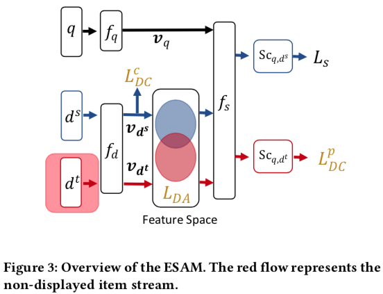
ESAM’s overall structure is shown below. Symbol meanings (basically concepts involved in vector retrieval):
- \(q\): query
- \(d^s\): exposed item
- \(d^t\): unexposed item
- \(f_q\), \(f_d\): functions mapping query and item to embeddings
- \(v_{q}\), \(v_{d}\): embeddings mapped by \(f_q\), \(f_d\)
- \(f_s\): function computing similarity between \(v_{q}\) and \(v_{d}\), commonly inner product
- \(L_s\): loss function based on prediction \(S_{c_{q,d^s}}\) from \(f_s\), common types include point-wise, pair-wise, list-wise
- \(L_{DA}\), \(L_{DC}^{c}\), \(L_{DC}^{p}\): three approaches proposed in the paper to mitigate exposure bias, added as losses to the original \(L_s\), detailed below
ESAM’s core lies in the three terms added to the original loss \(L_s\): \(L_{DA}\), \(L_{DC}^{c}\), \(L_{DC}^{p}\). Below we describe each term’s meaning and calculation.
\(L_{DA}\): Domain Adaptation with Attribute Correlation Alignment
The motivation for this loss term is that the correlation between two features should be consistent in source and target domains. As shown below, the left figure considers price to have strong correlation with brand, brand to have moderate correlation with material, and price to have weak correlation with material. \(L_{DA}\) is based on the following two assumptions:
- Correlations are consistent in source and target domains
- Original features (price, brand, material) are mapped to certain dimensions in the embedding
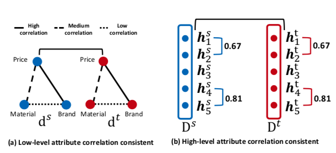
Therefore, we can design a loss term to make correlations between two features as consistent as possible in source and target domains. Correlation can be measured using covariance.
\(L_{DA}\) is calculated as follows. Let \(D^{s} = \lbrack v_{d_1^s};v_{d_2^s};\dots v_{d_n^s} \rbrack \in \mathbb{R}^{n×L}\) be the embedding matrix from n source domain samples, and \(D^{t} = \lbrack v_{d_1^t};v_{d_2^t};\dots v_{d_n^t} \rbrack \in \mathbb{R}^{n×L}\) be the embedding matrix from n target domain samples, where each \(v\) is a length-\(L\) vector.
If we extract the same dimension from each embedding as a vector \(h\), then \(D^{s}\) and \(D^{t}\) can also be written as follows, where each \(h\) is a length-\(n\) vector:
\(D^{s}=\lbrack h_{1}^{s},h_{2}^{s};\dots h_{L}^{s} \rbrack \in \mathbb{R}^{n×L}\)
\(D^{t}=\lbrack h_{1}^{t},h_{2}^{t};\dots h_{L}^{t} \rbrack \in \mathbb{R}^{n×L}\)
\(L_{DA}\) is calculated as:
\[\begin{align} L_{DA} &= \frac{1}{L^2}\sum_{(j,k)}({h_j^s}^T{h_k^s} - {h_j^t}^T{h_k^t})^2 \notag \\\ &= \frac{1}{L^2} ||Cov(D^s) - Cov(D^t)||_F^2 \notag \end{align}\]
Where \(Cov(D^s) \in \mathbb{R}^{L×L}\) and \(Cov(D^t) \in \mathbb{R}^{L×L}\) represent the covariance matrices of source and target domains. Note: the formula above is not entirely accurate because covariance calculation requires subtracting the mean, which isn’t done above.
After adding this term, the distribution of source and target domains in the vector space changes as follows: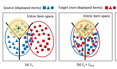
\(L_{DC}^{c}\): Center-Wise Clustering for Source Clustering
The second loss term \(L_{DC}^{c}\) is very similar to center loss first proposed in face recognition. It makes samples of the same type as close as possible in vector space. In advertising scenarios, types can be click, non-click, purchase, etc. Additionally, it makes samples of different types as far apart as possible. This idea is intuitive.
To define distance, a cluster center is defined for each type and parameterized. The calculation is:
\[\begin{align} L_{DC}^{c} &= \sum_{j=1}^{n} \max(0, ||\frac{v_{d_j^s}}{||v_{d_j^s}||} - c_{q}^{y_j^s}||_{2}^{2} - m_1) \notag \\\ &+ \sum_{k=1}^{n_y} \sum_{u=k+1}^{n_y} \max(0, m2 - ||c_{q}^{k} - c_{q}^{u}||_{2}^{2})\notag \end{align}\]
In the formula above, \(m_1\) and \(m_2\) are two margins, meaning no optimization is needed when the sample distance to its cluster is less than \(m_1\) or when cluster distance is greater than \(m_2\). Assuming all samples have \(n_y\) types, the center for type \(k\) (samples with label \(Y_k\)) is \(c_{q}^{k}\), defined as the center of vectors from current training samples of type \(k\):
\[\begin{align} c_q^k = \frac{\sum_{j=1}^{n} \delta(y_j^s = Y_k)\frac{v_{d_j^s}}{||v_{d_j^s}||}}{\sum_{j=1}^{n} \delta(y_j^s = Y_k)} \end{align}\]
After adding \(L_{DC}^{c}\), the distribution of source and target domains changes as shown below. Although target domain samples have high intra-cluster cohesion, their clusters might be wrong because no label information has been added for target domain samples yet. This is what the next loss \(L_{DC}^{p}\) addresses.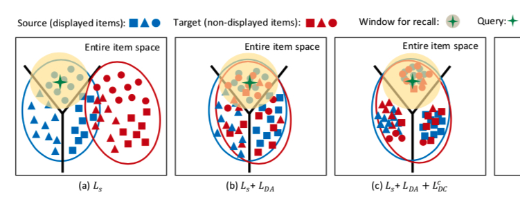
\(L_{DC}^{p}\): Self-Training for Target Clustering
From the self training in this loss’s description, we can guess it labels unlabeled target domain samples for model training, a common approach in semi-supervised learning. The paper doesn’t directly label unlabeled samples but cleverly achieves this through loss \(L_{DC}^{p}\):
\[\begin{align} L_{DC}^{p} = -\frac{\sum_{j=1}^{n} \delta(S_{c_{q,d^t}} < p_1 | S_{c_{q,d^t}} > p_2)S_{c_{q,d^t}} \log S_{c_{q,d^t}}} {\sum_{j=1}^{n} \delta(S_{c_{q,d^t}} < p_1 | S_{c_{q,d^t}} > p_2)} \end{align}\]
Where \(p_1\) and \(p_2\) are two thresholds, meaning only samples with confidence reaching a certain level are considered negative/positive. This loss makes samples with predictions less than \(p_1\) have predictions closer to 0, and samples with predictions greater than \(p_2\) have predictions closer to 1. The reason can be seen in the plot of \(-p(x) \log p(x)\) below; minimizing this term achieves the self-training goal: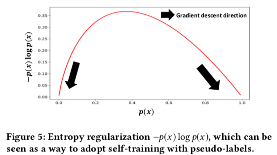
After adding \(L_{DC}^{p}\), the distribution of source and target domains changes as shown below, which is ESAM’s final form: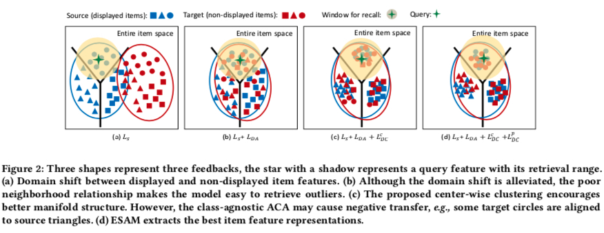
The final loss is shown below, where \(\lambda_1\), \(\lambda_2\), \(\lambda_3\) are three hyperparameters, solvable through gradient descent:
\[\begin{align} L_{all} = L_s + \lambda_1 L_{DA} + \lambda_2 L_{DC}^{c} + \lambda_3 L_{DC}^{p} \end{align}\]
Summary
In summary, this article mainly introduces three approaches for exposure bias: Data Augmentation, IPS, and Domain Adaptation. The main ideas are:
- Data Augmentation: Utilizing unlabeled samples through methods like treating all as negative, training an imputation model, or multitask learning
- IPS: Using only exposed samples, deriving from probability theory that properly weighted exposed samples give unbiased expectation
- Domain Adaptation: Utilizing unlabeled samples, mainly analyzing ESAM paper, which adds three loss terms to make the vector spaces learned from exposed and unexposed items as consistent as possible
While these methods look theoretically fancy, based on the author’s experience, applying them in practice requires considering model iteration efficiency, whether theoretical assumptions match reality, etc. For example, data augmentation/ESAM methods significantly increase data volume, which inevitably increases training time. Even if effective, we must consider whether the tradeoff between benefit and sacrificed iteration efficiency and machine resources is worthwhile, or consider improving sampling strategies to balance sample counts.