Dynamic Creative Optimization in Online Display Advertising

Posted on 2022-02-01 标签计算广告

Recently I’ve been researching creative-related content. Based on current investigation, I divide this field into three main parts: creative generation, creative selection, and creative delivery, with specific responsibilities as follows:

Creative generation: Using materials (titles, images, videos, landing pages, etc.) to generate candidate creatives (the ads users see)
Creative selection: Selecting top-k creatives from a campaign’s candidates (a campaign typically has multiple candidates) for delivery
Creative delivery: Delivering the selected creatives online

Strictly speaking, these three parts are not clearly demarcated. For example, the first two can be unified as creative generation (generating final delivery creatives from raw materials), and the latter two can be unified as creative delivery (selecting from candidates and delivering online).

This article mainly focuses on a paper related to creative delivery, particularly the third part (without E&E-based selection). The paper title is Dynamic Creative Optimization in Online Display Advertising. This paper models the online delivery problem as a bipartite graph matching problem, providing both exact and approximate online solutions. More importantly, this modeling approach is not limited to the creative domain and can be applied to many delivery scenarios.

Problem Modeling

Most methods in online advertising, such as targeting, ranking, and bidding, essentially solve the online allocation problem: distributing suitable ads to suitable users to maximize revenue (while considering ecosystem and user experience). Therefore, we can construct a simple bipartite graph as shown below, where the left side represents users and the right side represents specific ads (creatives here). The connecting edges indicate that a user accessed an ad/creative, and edge weights can be determined by specific business objectives.

Based on the bipartite graph above, the paper models the problem as the following optimization problem: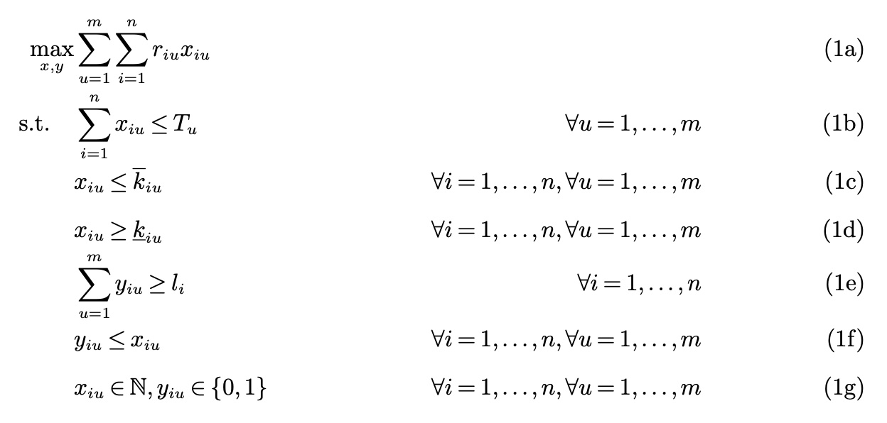

Symbol meanings are as follows:

\(u\): user index
\(i\): item index, where item refers to creative
\(r_{iu}\): revenue from the \(u\)-th user accessing the \(i\)-th item, such as cost/clicks, i.e., the edge weight in the figure above
\(T_u\): total number of accesses by the \(u\)-th user
\(x_{iu}\): number of times the \(u\)-th user accessed the \(i\)-th item
\(\underline{k_{iu}}\): lower bound on the number of times the \(u\)-th user accesses the \(i\)-th item
\(\overline{k_{iu}}\): upper bound on the number of times the \(u\)-th user accesses the \(i\)-th item
\(y_{iu}\): whether the \(u\)-th user accessed the \(i\)-th item
\(l_i\): lower bound on the number of different users reached by the \(i\)-th item (to prevent showing ads to only one user)

The three constraints (1b) to (1d) in the optimization problem correspond to the following three constraints:

(1b) ad fatigue constraint, which aims to help in avoiding customers becoming fatigued by seeing a product too many times. This constraint says that a particular item \(i\) can be shown at most \(\overline{k_{iu}}\) times to user \(u\). To calibrate ad fatigue, this parameter can be set using historical data showing when customers stop engaging with ads. (1c) ad retargeting constraint, which focuses on showing products to customers that have seen or searched for them before. In this constraint, we say that a particular item \(i\) has to be shown at least \(\underline{k_{iu}}\) times to user \(u\). To retarget an ad, this parameter can be set positive for items that the user saw just before the ad campaign is planned. (1d) user diversity constraint, which addresses the requirement that advertisers want to increase reach and purchasing by showing their products to many different customers. This constraint says that at least \(l_i\) users have to see a particular item \(i\). These parameters are specifically set by the advertiser.

Problem Solving

The problem solving is divided into offline and online parts. The difference is that offline we have a god’s-eye view of the problem, i.e., we can obtain user access counts \(T_u\), but online we don’t know them. Therefore, offline can use exact methods, while online must use approximate methods.

Offline Solving

If we can obtain \(T_u\) (i.e., user access counts for the day), we can solve the optimization problem above. Such problems are typically transformed into network flow problems. For a more detailed introduction to network flow, see Algorithm Learning Notes (28): Network Flow.

The problem modeled above can be transformed into a minimum-cost flow problem in network flow. For more details, see Algorithm Learning Notes (31): Minimum-Cost Maximum Flow.

Based on the minimum-cost maximum flow concept, we can construct the following network flow: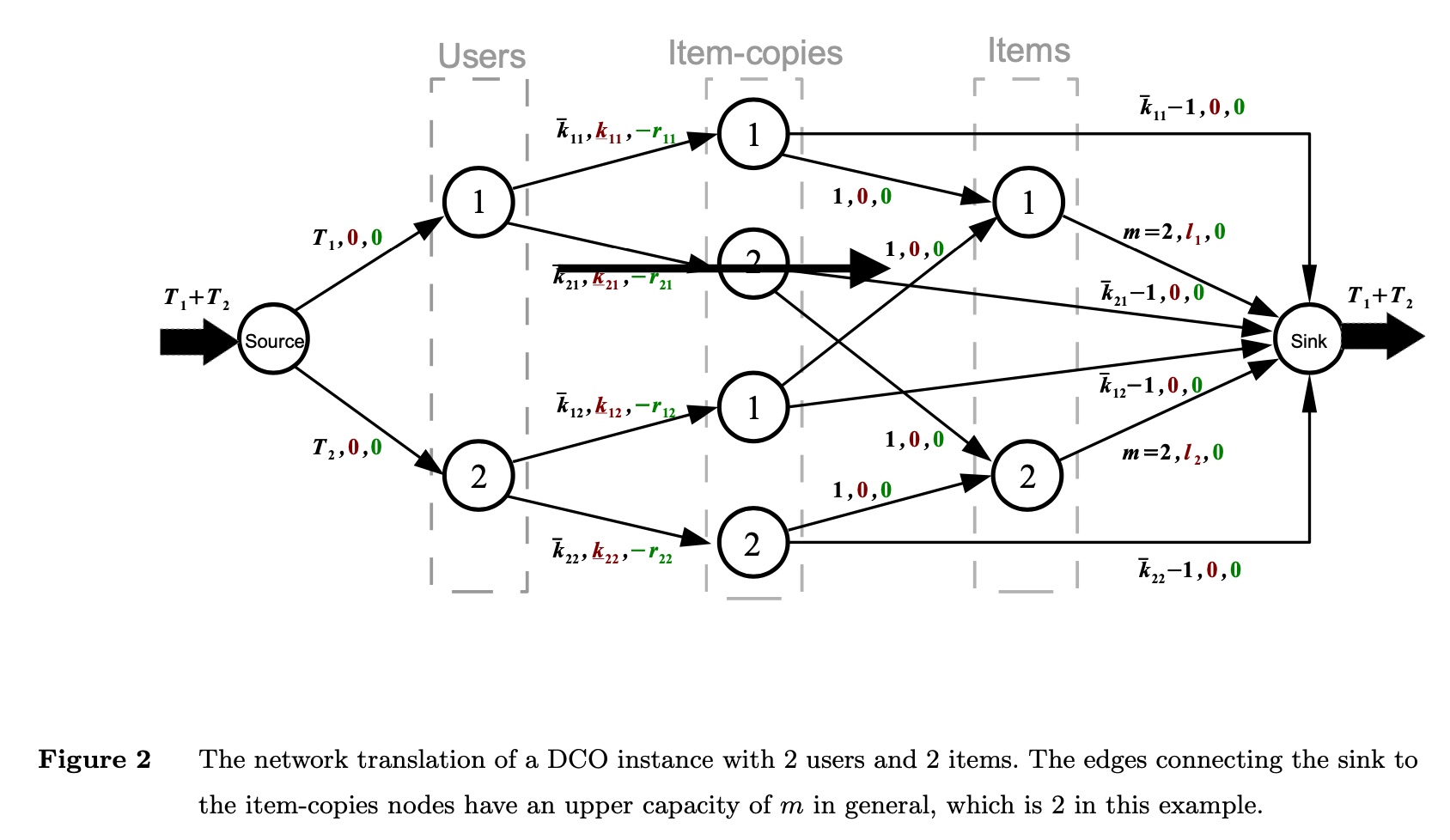

The network flow above has 2 users and 2 items. Understanding the following points will help you understand the figure:

The three parameters on each edge represent (flow upper bound, flow lower bound, cost)
The flow upper bound from source to the \(u\)-th user is \(T_u\) (i.e., the user’s current number of accesses)
The upper bound (ad fatigue constraint) and lower bound (ad retargeting constraint) for each user’s access to each item are reflected in the edges from users->item-copies
The edges from item-copies->items satisfy the user diversity constraint, ensuring the number of different users accessing the \(i\)-th item is not less than \(l_i\)
In item->sink, the flow upper bound is \(m\), meaning the upper bound on different users accessing the \(i\)-th item is the total number of users

Additionally, the following issues need to be considered in the graph construction. The paper doesn’t give clear answers; these are relatively open problems that need specific technical solutions for different business scenarios:

(1) What is the physical meaning of edge weights (i.e., the negative of cost mentioned above)? How to calculate weights for missing edges? (2) If the id granularity is too small, the entire graph might be too large, making graph solving difficult. How to do clustering? (3) How to handle new uid/item-id?

Online Solving

The above solution is offline, where we have the user’s daily access count \(T_u\) and can solve the optimization problem exactly. This mode can be used to estimate the upper bound of the method’s benefit (by replaying historical ranking logs). But in actual delivery, we don’t know the user’s daily access count \(T_u\) (Author’s note: if using historical average to approximate, how large would the error be?), so we need an approximately optimal online solution.

deterministic algorithm

The paper points out that deterministic algorithm (simply put, algorithms without random operations, unlike heuristic algorithms) performs poorly for online problems. As for how poorly, the paper provides some proofs. Here we’ll skip the process and only give some core concepts and conclusions.

The paper uses competitive ratio to measure the effectiveness of deterministic algorithms. This metric mainly describes how much worse an online algorithm performs compared to offline in extreme cases. Quoting the definition from these lecture notes:

The competitive ratio of an online algorithm for an optimization problem is simply the approximation ratio achieved by the algorithm, that is, the worst-case ratio between the cost of the solution found by the algorithm and the cost of an optimal solution.

With the competitive ratio concept, the paper gives the following conclusions for deterministic algorithms (detailed proof in Section 4.1 of the paper):

Proposition 1. The competitive ratio of any deterministic algorithm for the online DCO problem is arbitrarily small
Proposition 2. Suppose that the revenue associated to all item and user pairs are bounded, that is, there exists an \(r\) such that \(\underline{r} ≤ r_{iu} ≤ 1\) for all items \(i\) and users \(u\). In this case, the competitive ratio of any deterministic algorithm for the online DCO problem is \(\underline{r}\)

deterministic algorithm with assumption

The above results have no assumptions. So the paper adds an assumption: user \(u\) has at least \(c_u\) accesses per day. The paper cites a conclusion from IAB (Interactive Advertising Bureau), claiming this data is relatively easy to obtain:

Using historical data, advertisers can make accurate estimates about the minimum number of times they expect a user to visit the platform during the advertising period (Interactive Advertising Bureau 2020).

However, the reference provided by the paper only lists some statistical data without mentioning the derivation of this conclusion… Logically, the author guesses that while the exact access count \(T_u\) for user \(u\) is hard to predict, the lower bound \(c_u\) might be easier to obtain.

With the assumption that \(c_u\) is easily obtainable, the paper provides the first online algorithm with the overall flow shown below: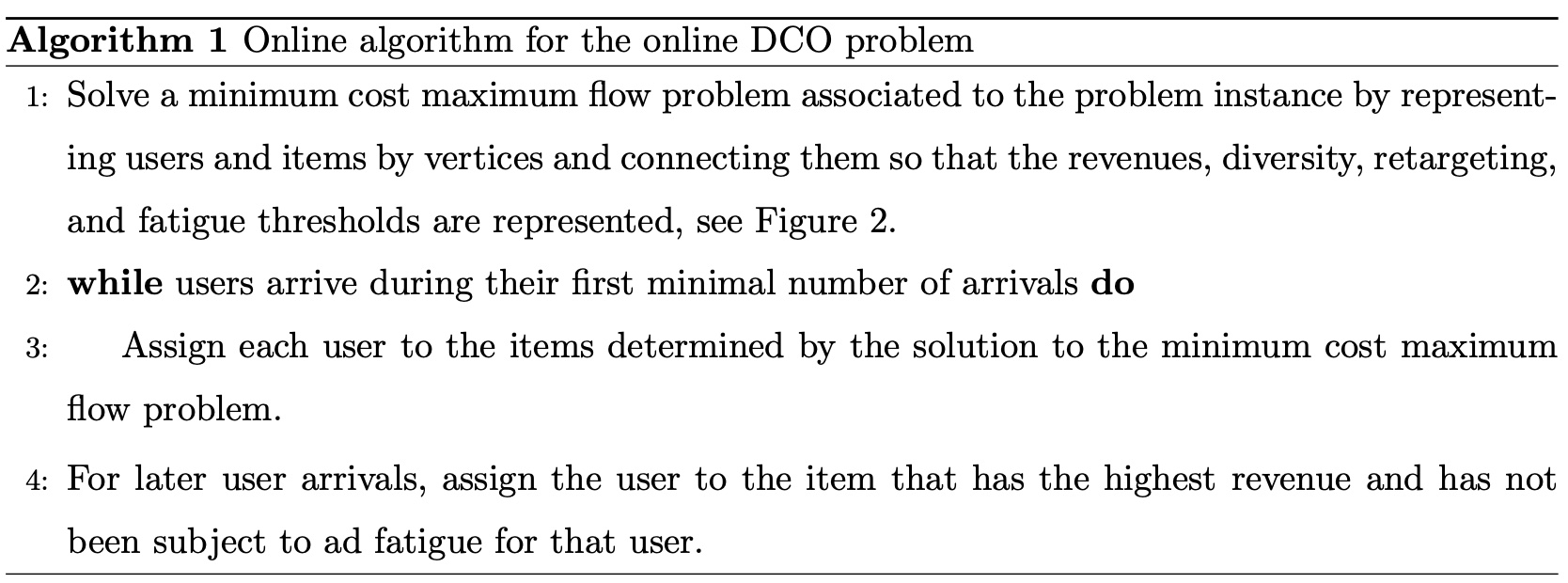

It’s not much different from offline, just using \(c_u\) instead of \(T_u\). During online allocation, constraints are satisfied first, then after satisfying constraints, the edge with highest revenue is selected within the ad fatigue constraint.

The paper goes through a long detour before giving this algorithm flow, with various symbols, lemmas, and propositions that don’t have much to do with the final conclusion, feeling like padding. And the core part of how to obtain \(c_u\) is barely mentioned…

The paper also gives a lower bound for this algorithm’s competitive ratio (proof in the paper, omitted here):

\[\begin{align} 1-\frac{(\overline{r} - \underline{r})n_1}{\underline{r}(n_1+n_2)} \end{align}\]

Symbol meanings:

\(n_1=\sum_{u=1}^{m} c_u\): sum of minimum access counts for all users
\(n_2= T- n_1\): \(T\) is the sum of actual access counts for all users
\(\underline{r}=\min_{i=1 \dots n, u=1 \dots m}r_{iu}\): minimum revenue across all pairs
\(\overline{r}=\max_{i=1 \dots n, u=1 \dots m}r_{iu}\): maximum revenue across all pairs

greedy algorithm

The paper also mentions another greedy algorithm with the assumption that each item/user has a reserved revenue. The \(i\)-th item’s reserved revenue is \(\alpha_i\), and the \(u\)-th user’s reserved revenue is \(\beta_u\), so:

\[\begin{align} r_{iu} = \alpha_i + \beta_u \end{align}\]

Based on this assumption, the paper provides the following online algorithm and proves its competitive ratio matches the optimal: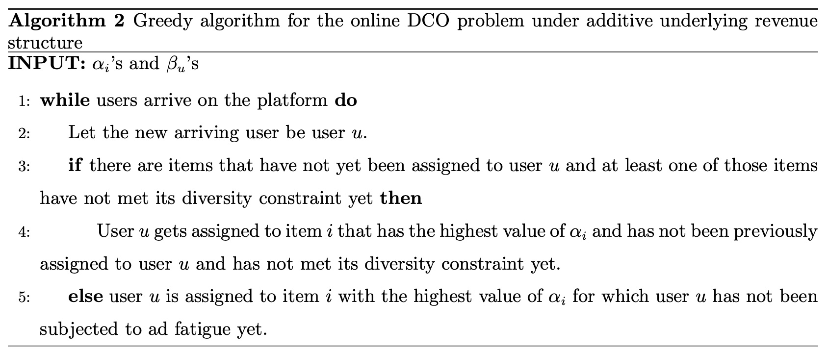

However, the author thinks this assumption has major problems: assuming each item has the same revenue for all users is clearly unreasonable. It’s precisely because each user has different interests that personalized recommendation is needed, which is why various algorithms and strategies work in current recommendation/advertising. So while this algorithm’s mathematical principles are worth studying, it’s not practical for real applications.

Summary

Overall, this paper models online ad allocation as a classic bipartite graph problem, providing both offline and online solutions with theoretical proofs. The author thinks the ideas are worth learning, but directly applying the paper’s methods in practice is difficult.

The first online algorithm’s problem is that obtaining \(c_u\) isn’t clearly specified. The second online algorithm’s problem is that the underlying assumption is unreasonable.

The author believes using user \(u\)’s past access counts to approximate (or predict) future access counts \(T_u\) is a feasible approach, but this method still needs to solve the following problems:

(1) If solving determines a certain item should be allocated to a certain user, the paper says to directly display it, but actual systems typically have a “retrieval + ranking” structure. How to ensure this item is definitely seen by the user? Or, actual systems already have retrieval and ranking strategies; how to integrate this new strategy into existing systems?

(2) What is the physical meaning of user-item edge weights? How to calculate weights for missing edges?

(3) Using id granularity might make the graph too large, making graph solving difficult. How to handle this? If doing clustering, how to ensure minimal difference between two clustering results?

(4) How to handle new uid/item-id?