A Hybrid Bandit Model with Visual Priors for Creative Ranking in Display Advertising
The previous article Dynamic Creative Optimization in Online Display Advertising mentioned that creative optimization can generally be divided into three main parts: creative generation, creative selection, and creative delivery. This article mainly covers some approaches for creative selection, which typically involves an exploration-exploitation (E&E) process.
This article is primarily based on a paper published by Alibaba: A Hybrid Bandit Model with Visual Priors for Creative Ranking in Display Advertising. The paper achieves the goal of ranking candidate creatives under the same campaign (i.e., creative selection) through list-wise training. List-wise can be considered as the exploitation part, while the paper also uses a bandit model for exploration. The overall approach is quite reasonable and has been validated in real-world industry scenarios, making it worth reading.
The method proposed in the paper mainly consists of two modules: VAM (visual-aware ranking model) and HBM (hybrid bandit model). The overall architecture is shown below. VAM is the exploitation module based on list-wise selection mentioned above, and HBM is the exploration module based on the bandit model. The following sections will introduce these two modules in detail.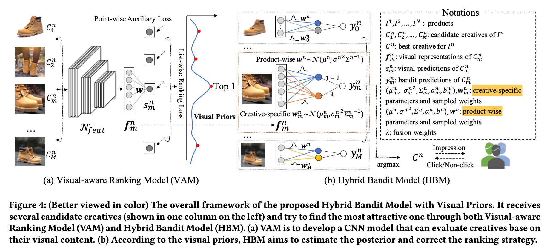
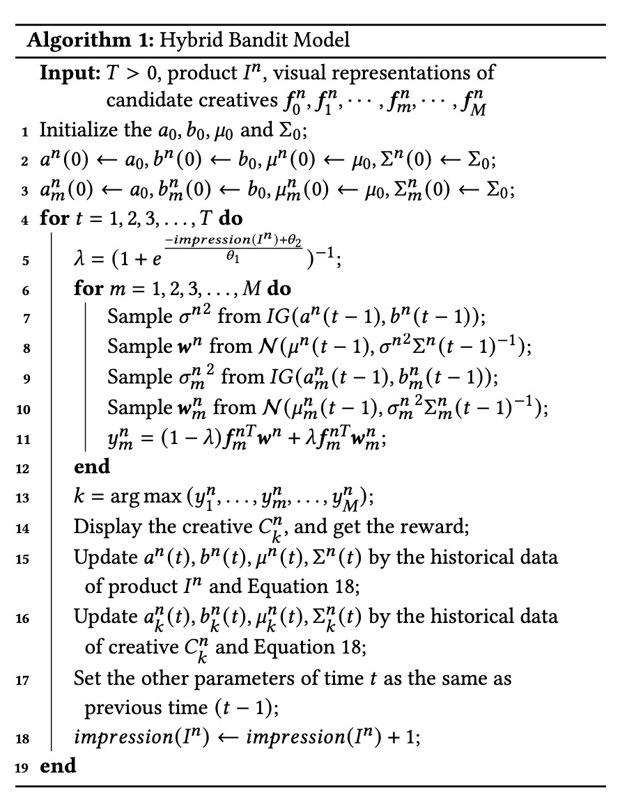
VAM
list-wise loss
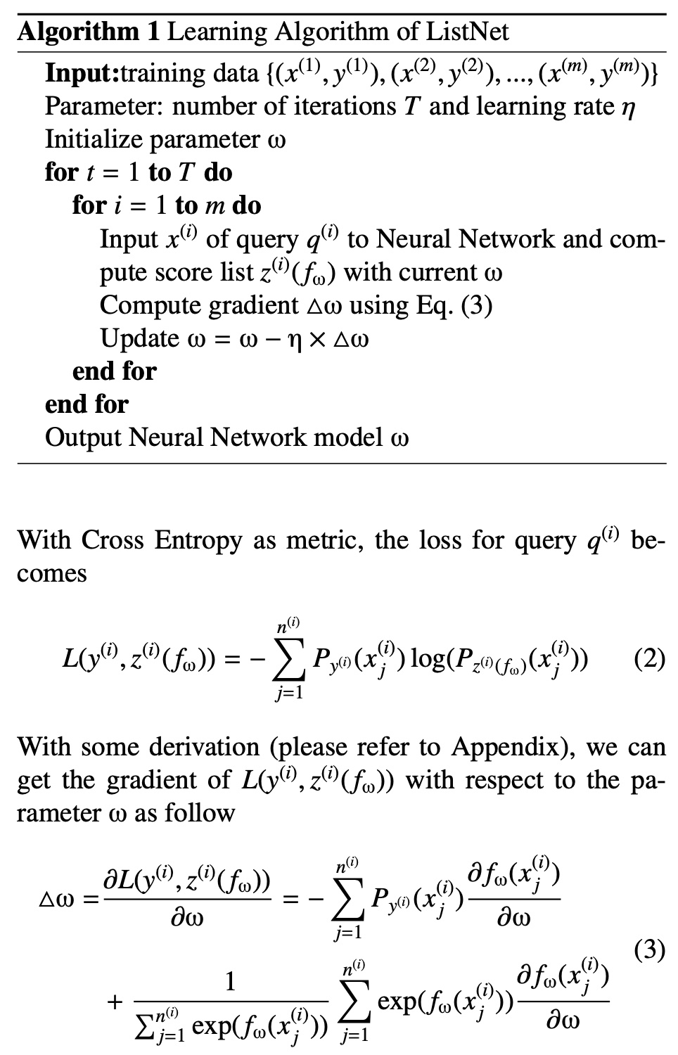
List-wise is a modeling approach in learning to rank. The other two approaches are point-wise and pair-wise. Common CTR/CVR prediction models use the point-wise approach.
For more details on these modeling approaches, refer to the following two papers, both published by Microsoft. The first paper describes the transition from point-wise to pair-wise, and the second paper describes the transition from pair-wise to list-wise.
- From RankNet to LambdaRank to LambdaMART: An Overview
- Learning to Rank: From Pairwise Approach to Listwise Approach
The list-wise loss used in VAM is the one proposed in the second paper. Its process is shown in the figure below. For more detailed derivation, please refer to the second paper above.
VAM loss
Returning to VAM, the query in the figure above corresponds to a product, while the list corresponds to all creatives for each product (a product typically has multiple candidate creatives).
Therefore, the prediction \(p_{m}^{n}\) and ground truth \(y_{rank}(C_m^n)\) for each item in the list are expressed as follows. The meaning of each symbol can be found in the upper right corner of the overall framework diagram above.
\[\begin{align} p_{m}^{n} = \frac{\exp(s_m^n)}{\sum_{i=1}^{M}\exp(s_i^n)} \end{align}\]
\[\begin{align} y_{rank}(C_m^n) = \frac{\exp(CTR(C_m^n), T) }{\sum_{i=1}^{M}\exp(\exp(CTR(C_i^n), T))} \end{align}\]
The \(T\) in \(y_{rank}(C_m^n)\) serves to adjust the scale of the value so that make the probability of top1 sample close to 1. Then for the \(n\)-th product, its list-wise loss is as follows:
\[\begin{align} L_{rank}^{n}=-\sum_{m}y_{rank}(C_m^n)\log(p_{m}^{n}) \end{align}\]
In addition to the conventional list-wise loss, the paper also adds a point-wise auxiliary regression loss. Its meaning is quite intuitive: it makes VAM’s predictions as close as possible to the actual CTR values, expressed as follows:
\[\begin{align} L_{reg}^{n}=\sum_{m} ||CTR(C_m^n) - s_m^n||_{2} \end{align}\]
According to the original paper, making the outputs close to the real CTRs will significantly stabilize the bandit learning procedure. Its purpose is to make the subsequent HBM training more stable. Thus, the overall loss for the \(n\)-th list is as follows (\(\gamma\) = 0.5 in experiments):
\[\begin{align} L^{n} = L_{rank}^{n} + \gamma L_{reg}^{n} \end{align}\]
noise mitigation
Noise mitigation here refers to the fact that some creatives have relatively few impressions, resulting in high variance in their posterior CTR (extreme cases include only one impression).
A crude method is to set a threshold for impressions, and items below the threshold are not used as training data. However, this may result in too little training data. The paper adopts the following two methods:
The first method is label smoothing, proposed in the paper Click-Through Rate Estimation for
Rare Events in Online Advertising. The idea is based on the Bayesian approach to give the number of clicks and CTR values a prior distribution. This way, even when encountering extreme values, there is distributional constraint, preventing the final value from being too unreasonable.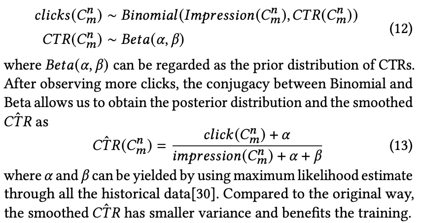
The second method is weighted sampling, which gives lower weight to samples with fewer clicks. The paper’s approach is to take the logarithm of the number of clicks as the weight for each sample.
HBM
HBM is essentially a Bayesian Linear Regression. As the name suggests, this is a Bayesian approach, which assumes that model parameters follow a distribution, and achieves exploration through sampling from the distribution. The derivation process is as follows:
Assume online data is generated as follows, where \(y\) represents whether a click occurred, \(f^T\) represents the visual representation extracted through VAM, and \(\widetilde{w}\) and \(\epsilon\) are the model parameters.
\[\begin{align} y = f^T\widetilde{w} + \epsilon \end{align}\]
The paper assumes the prior distribution of \(\epsilon\) as a normal distribution, i.e., \(\epsilon \thicksim N(0, \sigma^2)\). Similarly, \(\widetilde{w}|\sigma^2\) is assumed to be a normal distribution. They are conjugate to each other.
\[\begin{align} \sigma^2 \thicksim IG(a, b) \end{align}\]
\[\begin{align} \widetilde{w}|\sigma^2 \thicksim N(\mu, \epsilon^2 \Sigma^{-1}) \end{align}\]
Referring to the derivation process in the wiki above, the overall model training and serving process is shown below: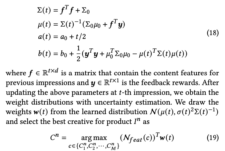
Formula 18 can be considered as the training process (in Bayesian methods, this has a specific name Bayesian inference). In Bayesian methods, updating the model means updating the parameters in the assumed distribution. In this example, the parameters are \(a\), \(b\), \(\mu\), and \(\Sigma^{-1}\) in the two distributions above. Analytical methods are used here, but for many problems, analytical solutions are not available, so Monte Carlo sampling methods are often utilized.
Serving involves sampling \(w(t)\) from the distribution obtained during training to calculate the final score.
The above method for calculating scores uses one set of parameters \(w^n\) for all creatives under the \(n\)-th product. The paper also proposes that each creative should have its own parameters, meaning for the \(m\)-th creative under the \(n\)-th product, the calculated score should be:
\[\begin{align} y_m^n = {f_m^n}^{T}w^n + {f_m^n}^{T}w_m^n \end{align}\]
The paper’s rationale for this is:
This simple linear assumption works well for small datasets, but becomes inferior when dealing with industrial data. For example, bright and vivid colors will be more attractive for women’s top while concise colors are more proper for 3C digital accessories. In addition to this product-wise characteristic, a creative may contain a unique designed attribute that is not expressed by the shared weights. Hence, it is helpful to have weights that have both shared and non-shared components.
Therefore, the paper calculates a weight \(\lambda\) for the score based on impression count, calculated as follows:
\[\begin{align} \lambda = (1+e^{\frac{-impression(I^n)+\theta_2}{\theta_1}})^{-1} \end{align}\]
The final score is then:
\[\begin{align} y_m^n = (1-\lambda){f_m^n}^{T}w^n + \lambda{f_m^n}^{T}w_m^n \end{align}\]
The idea here is that when a product has sufficient impressions, we should trust its product-wise score more; conversely, we should trust the creative-wise score more.
However, the author has doubts about this approach. The author believes that the \(\lambda\) parameter should be at the creative granularity. When creative-level data is sufficient, we should trust the creative-wise score more; conversely, we should trust the product-wise score more.
Because if each creative has sufficient posterior data for training, achieving creative-level personalized parameters would be best. However, the reality is that many creatives have very sparse or no posterior data at all. In such cases, using the product-wise score is essentially doing clustering, which the author believes makes more sense.
Therefore, the HBM algorithm flow is shown in the figure below:
Experiments
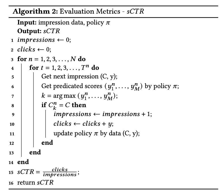
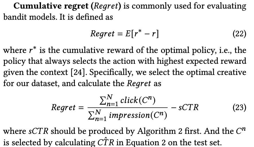
The paper used two evaluation metrics: Simulated CTR (sCTR) and Cumulative regret. The former simulates the online learning process, while the latter evaluates the bandit model. Their calculation methods are shown below, but these metrics don’t seem to be very common?
Two datasets were used for evaluation: one self-constructed and one public dataset. Naturally, the method proposed in the paper achieved the best results, but the paper did not conduct online A/B experiments. Approximate offline metrics still differ from online results.
Summary
Overall, this paper proposes a creative selection method consisting of VAM + HBM. The author believes the following points are worth learning:
- VAM utilizes post-delivery data (CTR) to learn the visual representation of creatives through list-wise methods
- HBM uses VAM’s visual representation through a bandit model to implement the exploration part, while considering the fusion of product-wise and creative-wise modeling and score prediction
However, the author also has doubts about the following points:
- When combining product-wise and creative-wise scores, the \(\lambda\) parameter only considers product-wise information and doesn’t properly reflect creative-wise weight, for reasons explained above
- Ad systems typically have a retrieval + ranking architecture, and ranking is usually at the creative level. The system proposed above may not integrate well into existing ad systems, but using the visual representation learned by VAM as a feature for the ranking model is a possible approach
- VAM can already rank candidate creatives for selection, so why do we still need HBM for exploration? Or what benefits does exploration bring? Based on the author’s experience, in ad systems, exploration means disrupting the distribution formed by the original system’s feedback loop, which often breaks the stable state formed by the Matthew effect, often causing revenue decline, while corresponding gains are improvements in ecosystem or faith-based metrics.