Highlight Detection In Video
Highlight Detection, literally high-light detection, is generally applied in images or videos. This article focuses on video scenarios, where the task is to find “highlight” segments from a long video. “Highlight” is a very broad definition, unlike CTR/CVR which have clear meanings. Highlight definition varies by scenario: for e-commerce livestream, highlight segments might be the time periods with highest GMV; for non-commerce livestream, highlights might be time periods with most viewers or gifts.
Highlight Detection has wide practical applications: video sites like iQIYI and Bilibili automatically play some segments when hovering over videos - these can be considered highlight segments. Mainstream livestream platforms provide replay tools with highlight segment candidates. Besides user-facing, advertisers/merchants also get similar products, such as Qianchuan, Kuaishou Jinniu platforms.
Highlight Detection is a research direction in academia, but academic research is limited to several manually annotated datasets and can’t be directly applied to production environments. The reason is the highlight definition varies by scenario, requiring different datasets. There are many Highlight Detection papers. This article mainly covers 2 papers closer to industry, focusing on highlight supervision signal definition, loss function design, and dataset acquisition.
TaoHighlight
This method comes from TaoHighlight: Commodity-Aware Multi-Modal Video Highlight Detection in E-Commerce
Proposed by Taobao in 2021, the overall model structure is shown below. The model isn’t complex: the left part extracts multi-modal features, the right part does fine-tuning through GCN based on extracted features and scores. The loss function consists of two parts: Loss_reg and Loss_ag.
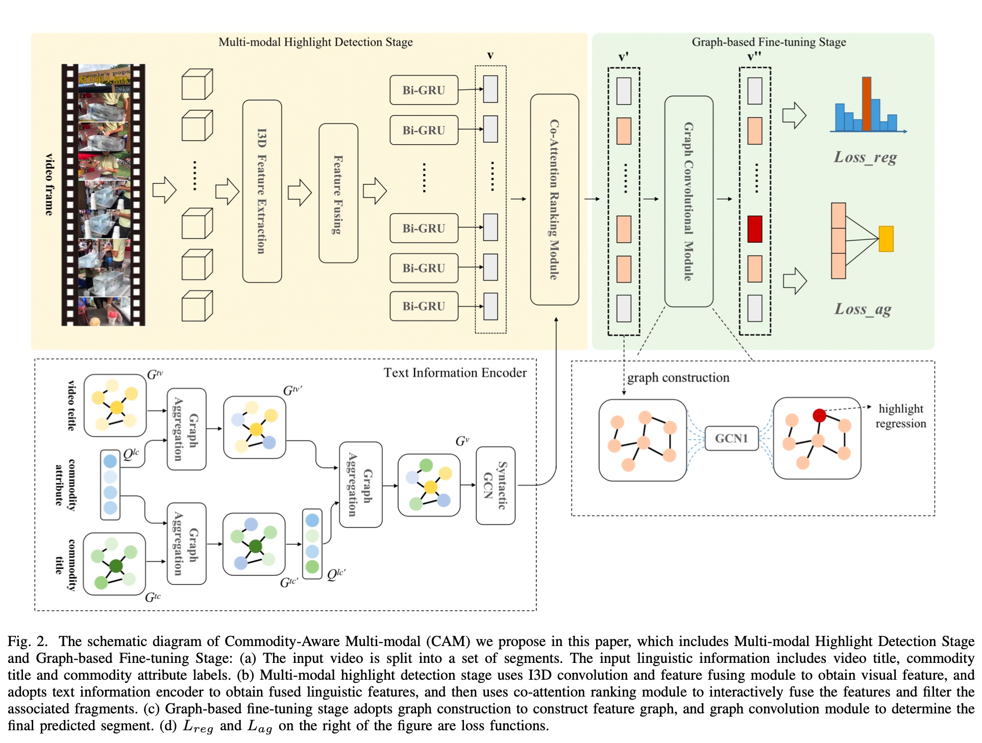
For feature engineering, visual information is extracted through I3D+BiGRU, quite conventional. Text information proposes QFGA (Query-Focus Graph Aggregation), a graph-based feature extraction module.
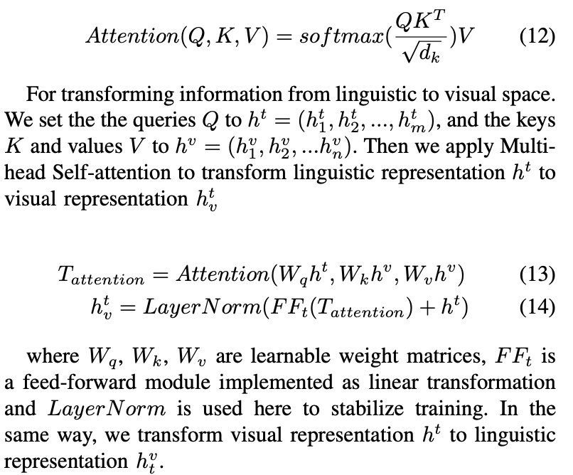
Co-Attention Module mainly fuses multi-modal features (visual and text information), with basic principle referencing transformer’s self-attention mechanism. For the left block below, \(v\) is query, \(s\) is key and value.
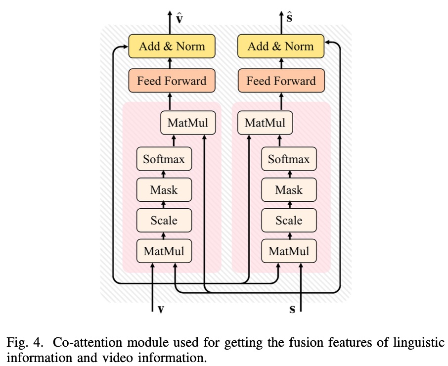
Its computation logic is shown below:
Graph-based Fine-tuning: This part mainly reduces noise in extracted features. The paper states: Due to the presence of visual and text noises in multi-modal video highlight detection, we propose a graph based fine-tuning module to improve the accuracy of our model. but doesn’t further explain.
The approach is to score each frame, select top-k frames by score to construct a graph, then do GCN computation. For detailed GCN explanation, see: Understanding Convolutions on Graphs.
The final loss function consists of 2 parts: \(L_{reg}\) and \(L_{ag}\), with meanings:
\(L_{reg}\) calculates the difference between predicted and actual start/end times:
\[\begin{align} L_{reg} = \frac{1}{N} \sum_{i=1}^{N}[R(\hat{s_i}, s_i) + R(\hat{e_i}, e_i)] \end{align}\]
Symbol meanings:
- \(s_i\), \(e_i\): predicted highlight segment start and end times
- \(\hat{s_i}\), \(\hat{e_i}\): ground truth start and end times
- \(R\): L1 function
\(L_{ag}\) calculates correlation between two video segments. \(k\) means cutting each video into \(k\) clips. It mainly consists of three terms:
\[\begin{align} L_{ag} = - \sum_{i=1}^{k}e(v_i, \hat{v}) \end{align}\]
\[\begin{align} e(v_i, v_j) = \theta_{r} \cdot r(v_i, v_j)+\theta_{d} \cdot d(v_i, v_j)+\theta_{s} \cdot \cos(v_i, v_j) \end{align}\]
Symbol meanings:
- \(v_i\), \(\hat{v_i}\): predicted highlight segment and ground truth
- \(r(v_i, v_j) = \frac{I(v_i, v_j)}{U(v_i, v_j)}\), is IoU metric, representing overlap ratio
- \(d(v_i, v_j) = \frac{ |c_i - c_j|}{U(v_i, v_j)}\), \(c_i\) and \(c_j\) represent centers of two videos
- \(cos\): cosine similarity between two segments
Prediction is a multi-class model (softmax), predicting on the final constructed graph, selecting the frame with highest probability as start, then taking the next 128 frames as the fixed highlight segment.
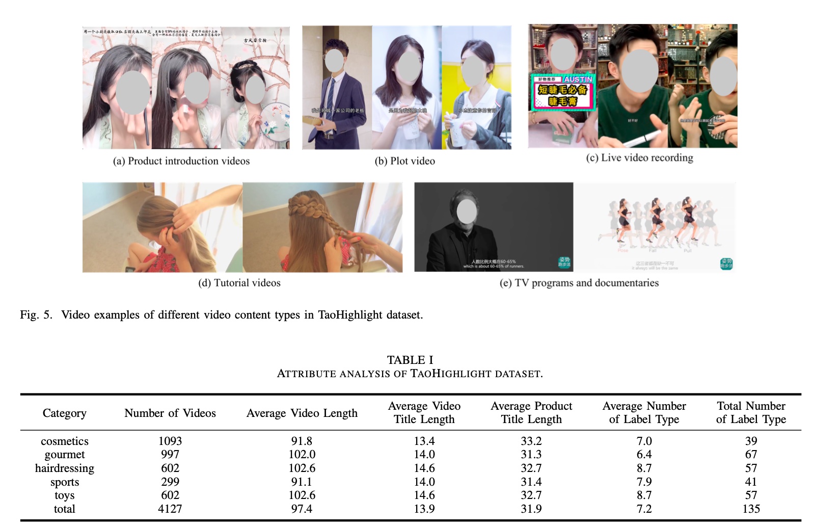
Experimental evaluation uses IoU metrics on a Taobao dataset with 5 major categories:
The paper does ablation studies:
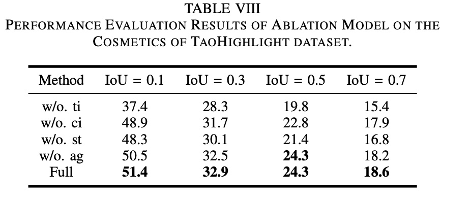
Symbol meanings below show text features, Graph-based Fine-tuning, and \(L_{ag}\) term in loss function have significant effects:
- w/o.ti. remove text features
- w/o.ci. text features only include video title (removed product title and attributes)
- w/o.st. removed Graph-based Fine-tuning
- w/o.ag. removed \(L_{ag}\) term in loss function
“unsupervised” solution
The TaoHighlight method above uses manually annotated datasets with obvious drawbacks: high annotation cost and poor maintainability. First, highlight definition varies by person, making annotation subjective. Second, cost and difficulty mean datasets update infrequently, unacceptable in industry.
So naturally we think: can we use unlabeled signals to avoid manual annotation? This paper provides an approach: Less is More: Learning Highlight Detection from Video Duration
The paper believes Less is More: shorter videos have higher information density, so segments can be considered highlights; conversely, longer videos have lower information density, segments aren’t highlights. Therefore, the paper divides training samples \(D\) into three parts: \(D= \lbrace D_S, D_L, D_R \rbrace\), where \(D_S\) is short video set, \(D_L\) is long video set. Videos shorter than 15s are defined as short, longer than 45s as long.
Each video is cut into equal-length segments, denoted \(s\), with \(v(s)\) indicating the video containing segment \(s\).
The paper uses pair-wise method to construct samples: take one segment each from \(D_S\) and \(D_L\) to form a pair \((s_i, s_j)\), then calculate difference using ranking loss. Ranking loss is actually a class of loss functions; common triplet loss, margin loss, hinge loss can all be considered ranking losses.
The loss function:
\[\begin{align} L(D) = \sum_{(s_i, s_j) \in \mathcal{P}} \max(0, 1 - f(x_i) + f(x_j)) \end{align}\]
But considering short video segments as highlights and long video segments as non-highlights is arbitrary, or contains noise, so we need confidence for each pair. A binary latent variable \(w_{ij}\) is introduced representing each pair’s confidence. The loss becomes:
\[\begin{align} &L(D) = \sum_{(s_i, s_j) \in \mathcal{P}} w_{ij} \max(0, 1 - f(x_i) + f(x_j)) \\\ &\begin{array} \\\ s.t.& \sum_{(s_i, s_j) \in \mathcal{P}} w_{ij} = p|\mathcal{P}|, w_{ij} \in [0,1] \\\ &w_{ij} = h(x_i, x_j) \end{array} \end{align}\]
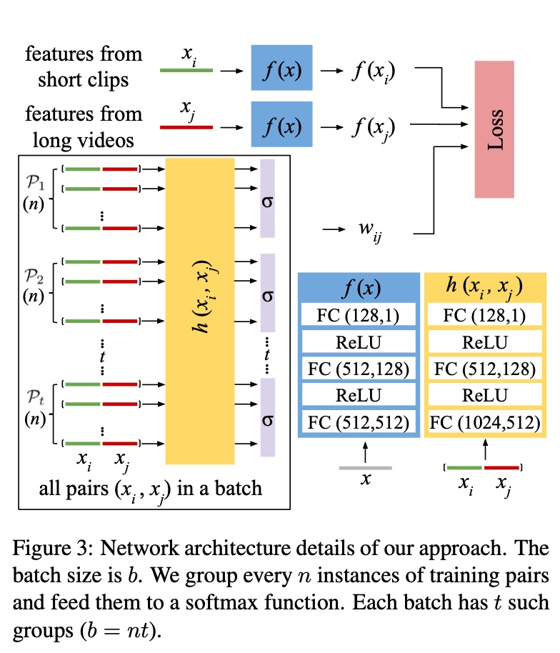
\(p\) represents the proportion of valid pairs in training samples, \(h\) is the network computing \(w_{ij}\), jointly trained with the original network during training. Actual implementation uses batch division + softmax.
Although \(w_{ij}\) makes only part of samples valid statistically, it may not completely eliminate noise because without manual prior information, \(w_{ij}\) might be smaller for truly valid pairs.
The overall model and process is shown below. \(\mathcal{P_1}\) to \(\mathcal{P_t}\) can be considered \(t\) batches, each with n pairs.
As mentioned above, \(w_{ij}\) actually works through batch division + softmax. The loss function becomes:
\[\begin{align} &L(D) = \sum_{g=1}^{m} \sum_{(s_i, s_j) \in \mathcal{P_g}} w_{ij} \max(0, 1 - f(x_i) + f(x_j)) \\\ &\begin{array}\\\ s.t.& \sum_{(s_i, s_j) \in \mathcal{P_g}} w_{ij} = \sum_{(s_i, s_j) \in \mathcal{P_g}} \sigma(h(x_i, x_j)) = 1 \\\ &w_{ij} \in [0,1] \end{array} \end{align}\]
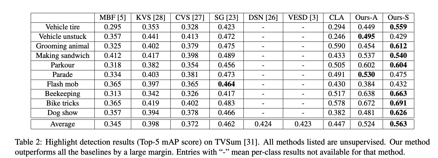
Experiments use mAP (mean average precision), common in object detection. It can be simply understood as: for each category in multi-category object detection, AP is the area under the PR curve, mAP is the mean across categories.
mAP definition is similar to AUC, but uses PR curve instead of ROC curve. See ROC Curve vs PR Curve for differences.
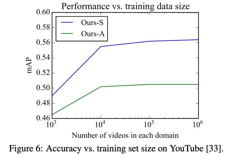
Experiments are on two public datasets: YouTube Highlights and TVSum. The datasets categorize videos by domain, so both overall modeling (Ours-A) and per-domain modeling (Ours-S) are tried. Results are good, even beating some supervised methods.

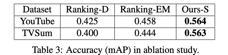
The paper also does ablation studies:
- For binary latent variable \(w_{ij}\), comparing removing \(w_{ij}\) (Ranking-D) and using EM to update \(w_{ij}\) (Ranking-EM): joint training > EM > removing \(w_{ij}\)
- Comparing dataset size effects: accuracy increases then slows as dataset grows, a conventional conclusion.
Summary
There are many papers on highlight detection. Here we selected two targeted papers with core points:
First paper: TaoHighlight: Commodity-Aware Multi-Modal Video Highlight Detection in E-Commerce
- Feature engineering: video and text feature extraction, fusion via co-attention
- Loss function design: \(L_{reg}\) + \(L_{ag}\)
- Noise reduction: graph-based fine-tuning for top-k candidates
Second paper: Less is More: Learning Highlight Detection from Video Duration
- Dataset: judging highlights from video length, no manual annotation
- Loss function design: pair-wise ranking loss
- Noise reduction: trainable binary latent variable for sample confidence
The second paper’s pattern feels more suitable for production environments, mainly because manual annotation has poor maintainability and sustainability. Building on the second paper, when actually deploying, several issues need consideration:
- Video duration is a coarse signal. In actual business, many metrics (CTR, CVR, ROI) might be better highlight definitions, while weighing signal depth vs data sparsity trade-off
- Besides ranking loss, LTR (pair-wise, list-wise) modeling is also a good choice; consider how to construct pairs or lists in practice
- For livestream scenarios requiring real-time highlight detection without access to the full video, consider streaming detection methods