A Brief Discussion on Computational Resource Optimization
Current recommendation or ad systems basically do request-level estimation and optimization, which brings the problem of rising machine costs while maximizing effectiveness. Uneven traffic distribution makes this problem more severe. For Douyin or Meituan, there are often two traffic peaks in a day: lunch peak and evening peak, because these are times when food ordering and phone scrolling increase dramatically. Traffic drops significantly in other time periods, as shown below.
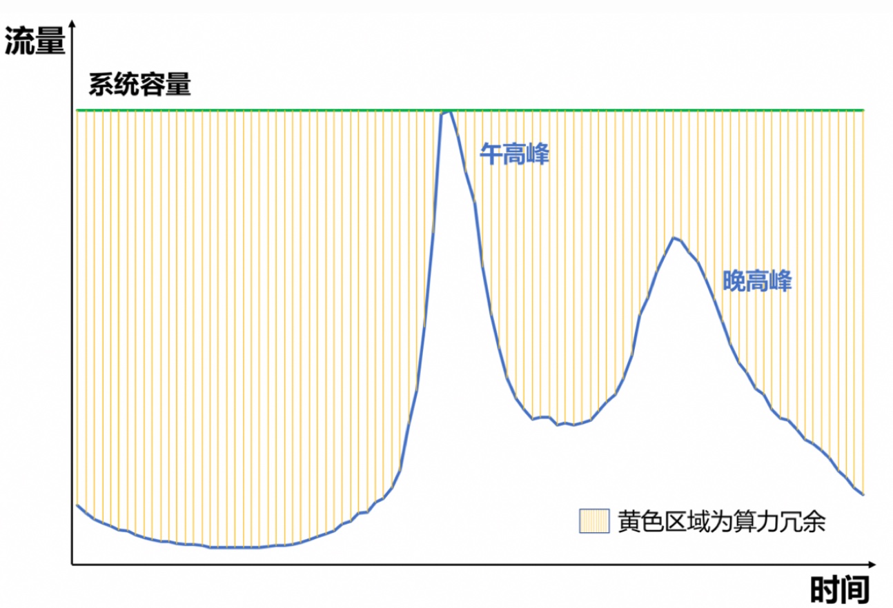
This means if we prepare enough machines to handle peak load, most machines are idling or have very low ROI in other time periods. Therefore, capacity expansion or degradation is often needed during peaks. Degradation generally means reducing request count by dropping traffic proportionally, but dropping traffic definitely hurts overall effectiveness. This has led to the research direction of computational resource optimization. Resource optimization is essentially a trade-off between effectiveness and machine cost, or how to reduce costs as losslessly as possible.
This article mainly introduces common approaches for computational resource optimization. I summarize them as drop, cache, and dynamic methods. If we decompose consumed computational resources, we can intuitively split into two parts: request count × computational cost per request. Therefore, we can optimize from these two aspects:
- drop: Directly drop traffic, i.e., directly reduce “request count”
- cache: Store previous estimation results in cache, so each estimation doesn’t need actual machine inference, i.e., reducing “computational cost per request”
- dynamic: Dynamically control computational cost per request based on request value. This method also reduces “computational cost per request”. DCAF is representative of this approach.
The above methods are all traffic-level optimization. There are also methods for optimizing model inference latency, mainly in computational parallelization (hardware upgrade), model compression (quantization, distillation, structure adjustment, etc.). This article won’t expand on these.
drop
Dropping traffic is the most primitive and crude degradation method, but it’s still effective and immediate in scenarios like traffic spikes. Besides crude indiscriminate traffic dropping, we can do this more precisely: through rule-based or model-based methods to determine whether to drop each request.
Rule-based methods often need to define invalid requests for specific business. For example, “invalid” in recommendation might be requests with no user clicks and short dwell time, in advertising might be no billing due to no impression. This way we can derive basic rules, like for users with n consecutive invalid requests, directly drop the next request.
Model-based methods are similar to rule-based, generally modeled as classification or regression problems. For classification, we need to clearly define positive and negative examples (i.e., invalid requests). For regression, we need to define each request’s value (like the estimation score used in final recommendation or advertising ranking).
A notable point is to keep the dataset unbiased or avoid feedback loop, we need to randomly allocate a portion from traffic without drop strategy enabled to generate training set (holdout dataset).
cache
Cache is also a common approach for saving computational resources. Previous request estimation results are cached, and when similar requests arrive, cached estimation results are returned directly. There are 2 key issues:
(1) Cache granularity - Generally finer granularity gives more accurate estimation, but consumes more KV storage. Common dimensions to consider include user, device, media position, access time, etc. Specific cache granularity can be cross-multiplied from several dimensions.
(2) Cache estimation bias - Since it’s not real-time estimation, estimation bias is often much higher than real-time estimation. The most intuitive solution is adding a calibration module on top of cache results (like Platt scaling). This issue is also related to cache TTL - generally larger TTL means larger estimation bias while consuming fewer resources. So keeping cache estimation bias small is meaningful for resource saving because TTL can be set longer.
This estimation bias manifests in posterior as generally overestimation, actually because underestimated traffic fails bidding and can’t get impression. This phenomenon has the same cause as the “small traffic overestimation problem” in many AB experiments. Actually it’s not just overestimation but estimation inaccuracy - we only see post-delivery data from overestimated delivery.
But the causes of estimation inaccuracy aren’t completely identical. The former is more from non-real-time nature, while the latter (small traffic overestimation) is essentially because 2 models simultaneously generate training datasets with different distributions (feedback loop). We can understand this as having 2 domains, then the model in small traffic domain uses data generated by large traffic domain model. Overall dominated by large traffic model data, can’t see its own overestimation (evidence: if we strictly isolate data for both models, this problem is greatly alleviated, but hurts overall performance because small traffic model has too little data, making traffic monetization efficiency low). So in practice, we often add domain-distinguishing features (like model name, rit) to the model, which can also alleviate the small traffic overestimation problem.
dynamic
Dynamic is the most researched method. The idea is intuitive: dynamically adjust computational cost per request based on each request’s estimated value. Higher value gets higher allocated computational cost, and vice versa.
Based on this idea, naturally there are 3 problems to solve: (1) request value estimation (2) computational cost estimation (3) allocation strategy.
For problem (1), in search/recommendation/advertising scenarios, there’s a ranking process, so we can approximate ranking score as traffic value. For recommendation, this value’s physical meaning might not be strong, but for advertising, eCPM-based ranking means actual revenue this traffic brings to the platform.
For problem (2), in the classic three-stage funnel of retrieval, coarse ranking, and fine ranking, we can measure computational cost by number of candidates entering each module. Notably: candidate count and computational cost are positively correlated but not linear, as will be detailed later.
For problem (3), after quantifying traffic value and computational cost, we can naturally model this allocation problem using optimization approach. The most common pattern is maximizing traffic value under computational cost constraint, with variable being candidate count for each request.
A representative work for allocation strategy is Alibaba’s 2020 paper DCAF: A Dynamic Computation Allocation Framework for Online Serving System. The paper mainly solves the third problem above. Let me first describe the paper’s allocation strategy, then discuss approaches for modeling traffic value and computational cost.
DCAF
Problem Modeling
The paper naturally models computational resource allocation as the following problem:

Symbol meanings above:
- \(i\): Request index
- \(j\): Action index, where action generally refers to candidate count entering each module
- \(x_{ij}\): Whether to take action j in request i, value 0 or 1. Each request can only take one action
- \(q_j\): Computational resource consumed by action j. Note the assumption is same action consumes same computational resource regardless of request
- \(Q_{ij}\): Value brought by action j in request i
- \(C\): Total computational resource limit
After modeling this problem, the paper mentions 2 important issues this modeling faces, which are actually common problems for this optimization paradigm.
First is needing to solve the optimization problem in real-time. This problem arises because when modeling this way, we assume we can get all data. If we collect data from past n days, we can do it, but in real-time online serving we can’t achieve this.
This problem is actually the same as optimization modeling in bidding scenarios. Reading Notes on “Bid Optimization by Multivariable Control in Display Advertising” is an example. The general approach in bidding is first deriving the optimal bid formula form through solving optimization problem, then determining unknown variables in the formula through real-time control. Later when discussing this problem’s solution, we’ll find this paper’s approach is somewhat different - needing to directly solve for the final solution.
Second is calculating traffic value \(Q_{ij}\). The paper suggests estimating through models and proposes the model needs to be lightweight enough because traffic-level estimation QPS is quite high.
Problem Solving
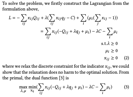
Problem solving uses Lagrangian duality method. For this method’s principle, refer to the Lagrangian duality section in Convex Optimization Summary. According to theory, we can write the above optimization problem’s Lagrangian dual problem as formula (3) below:
Unlike bidding derivation where we only need to get optimal bid formula without specific solution, so we can directly derive optimal bid formula by setting derivative to 0 for the variable. See Reading Notes on “Bid Optimization by Multivariable Control in Display Advertising” for detailed process.
But here we need to make specific decision or get specific solution, i.e., which action to choose for request i, which means which \(x_{ij}\) should be 1. So we need to solve this problem. The paper’s derivation:
Below is my understanding of the derivation steps:
Only when \(-Q_{ij} + \lambda q_j + \mu_i \ge 0\) does formula (3) have a lower bound (I don’t fully understand this, because here \(x_{ij}\) takes value 0 or 1, not arbitrary integer, so even if \(-Q_{ij} + \lambda q_j + \mu_i \lt 0\), there won’t be no lower bound (negative infinity))
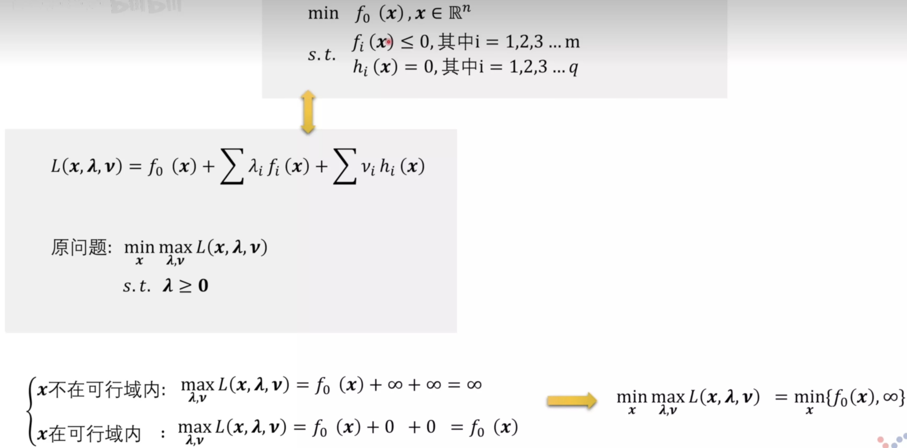
With condition \(-Q_{ij} + \lambda q_j + \mu_i \ge 0\), we can remove the min constraint. In formula (4) above, because at this point taking min will definitely make \(x_{ij}(-Q_{ij} + \lambda q_j + \mu_i)\) term 0. This is actually similar to deriving Lagrangian dual, as shown below (source):
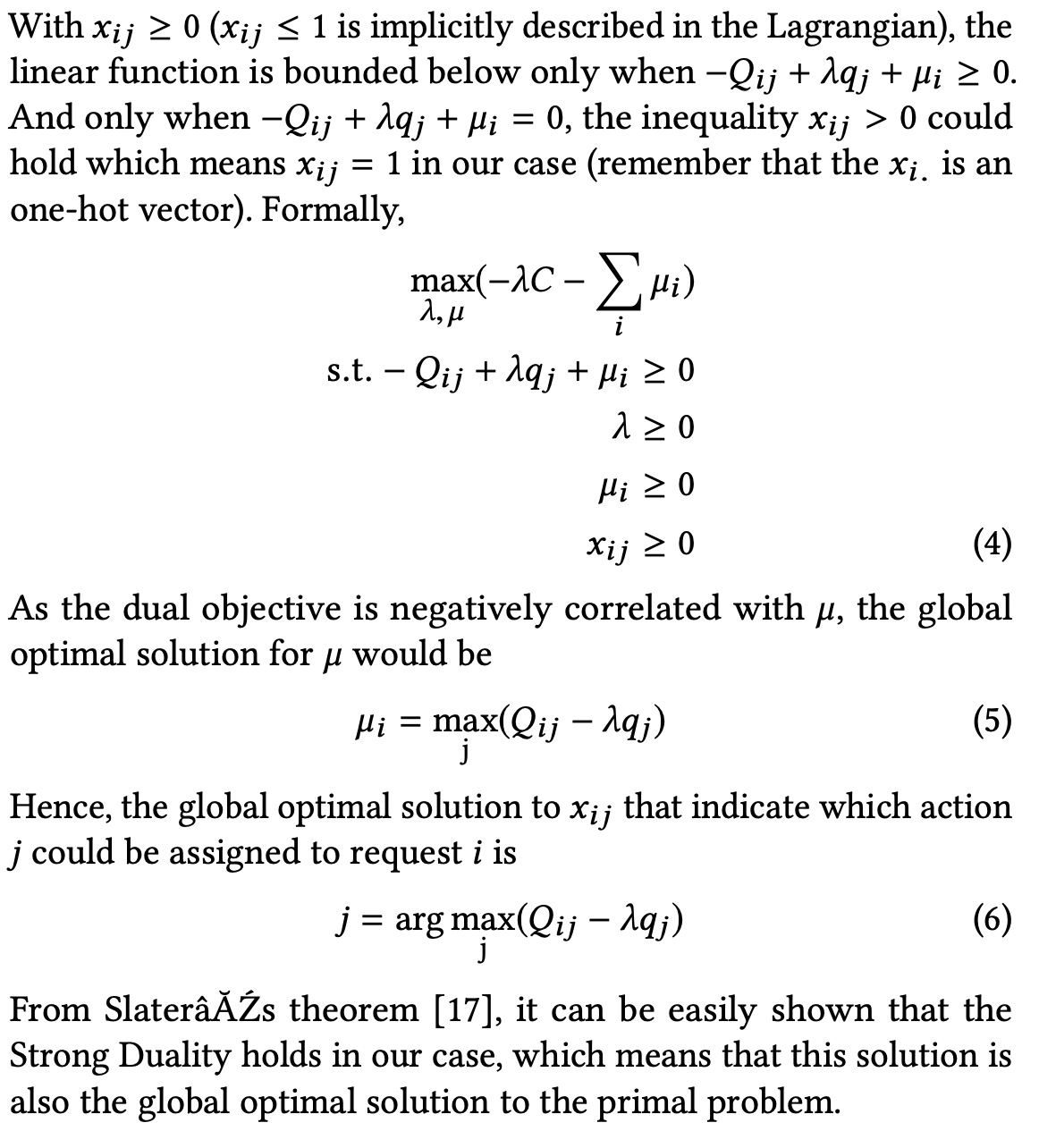
After removing min constraint, remaining max problem variables are \(\lambda\) and \(\mu\). From constraint \(-Q_{ij} + \lambda q_j + \mu_i \ge 0\), we can derive \(\mu_i \ge Q_{ij} - \lambda q_j\), i.e., the maximum of \(Q_{ij} - \lambda q_j\) across all actions for request i should be less than \(\mu_i\). Since it’s a max problem and negatively related to \(\mu_i\), \(\mu_i\) should be as in formula (5).
Therefore, for request \(i\), the actually effective constraint is \(\max_j (Q_{ij} - \lambda q_j)\) (this constraint is tight). Only at this point is \(x_{ij}\) not 0, i.e., the final action (see formula (6)).
From formula (6), for online serving, we still need to know \(\lambda\) value (\(Q_{ij}\) and \(q_j\) modeling methods discussed in next section).
But \(\lambda\)’s analytical solution is hard to find in this problem. The paper makes 2 assumptions:
Assumption 1: \(Q_{ij}\) monotonically increases as \(j\) increases Assumption 2: \(Q_{ij}/q_j\) monotonically decreases as \(j\) increases
Assumption 1 means more candidates brings more value from this traffic (I think we need to add constraint that online resources can handle it, otherwise more candidates might increase error rate and decrease traffic value. A MaxPower concept mentioned later in the paper addresses this). Assumption 2 means marginal return decreases as candidate count increases, which makes sense.
Based on these two assumptions, we can derive total computational resource \(\sum_{ij} x_{ij}q_j\) monotonically decreases as \(\lambda\) increases. See paper’s Section 4.2 for details. Here’s a more intuitive explanation: From formula (5) above, \(\max_j (Q_{ij} - \lambda q_j) \ge 0\), i.e., \(Q_{ij}/q_j \ge \lambda\). \(Q_{ij}/q_j\)’s physical meaning can be understood as unit computational resource return. From assumption 2, as computational resource or candidate count increases, marginal cost decreases. Therefore, as \(\lambda\) increases, meaning higher requirement for computational resource cost, candidate count needs to decrease (this is also a physical meaning of \(\lambda\)).
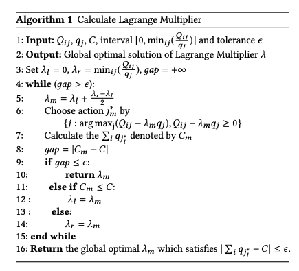
With the conclusion above that “total computational resource \(\sum_{ij} x_{ij}q_j\) monotonically decreases as \(\lambda\) increases”, we can find a \(\lambda\) through binary search that makes consumed computational resource just approach total resource quota \(C\), as shown in the algorithm below. Line 11’s symbols seem reversed.
System Design
DCAF’s overall framework is shown below. Left part mainly models \(Q_{ij}\), right part is online serving system.
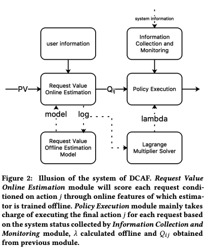
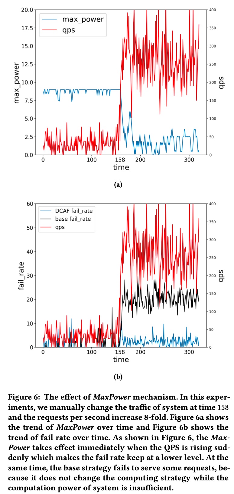
Left part is straightforward. Let me focus on right part. The upper right “Information Collection and Monitoring” part collects real-time data on current system load like error rate, timeout rate, etc., and controls error rate and timeout rate through PID algorithm, or controls current system’s sustainable upper limit to avoid system crash. The paper calls this MaxPower, which can be understood as adjusting each request’s candidate count upper limit based on system’s real-time load.
This is reflected in experimental setup - as system load QPS increases, MaxPower automatically decreases to ensure overall system stability, as shown below:
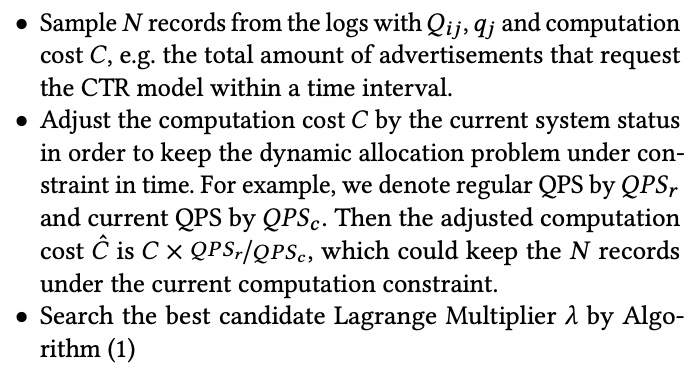
\(\lambda\) is calculated in real-time using binary search above, sampling data from a period. Algorithm’s capacity \(C\) is converted based on QPS. Offline \(\lambda\) calculation process:
Experimental Design
Experiments include offline and online parts.
Offline experiment mainly does traffic replay. \(\lambda\) is calculated as above. Computational cost \(q_j\) represents request candidate count. \(Q_{ij}\) represents sum of top-k ad eCPM under computational cost \(q_j\).
- Action \(j\) controls the number of advertisements that need to be evaluated by online CTR model in Ranking stage.
- \(q_j\) represents the advertisement’s quota for requesting the online CTR model
- \(Q_{ij}\) is the sum of top-k ad’s eCPM for request \(i\) conditioned on action \(j\) in Ranking stage which is equivalent to online performance closely. And \(Q_{ij}\) is estimated in the experiment.
Offline results shown below. Left y-axis eCPM is actual traffic value, right y-axis is actual computational cost consumed. Results show offline replay can decrease computational cost while increasing traffic value. As \(\lambda\) increases, DCAF’s total consumed computational cost and traffic value both decrease, consistent with \(\lambda\) derivation process above, because \(\lambda\)’s physical meaning is a threshold for marginal return of increasing candidates. As candidates increase, marginal return decreases, and when below \(\lambda\) is where to truncate candidate count, i.e., \(q_j\)’s specific value.
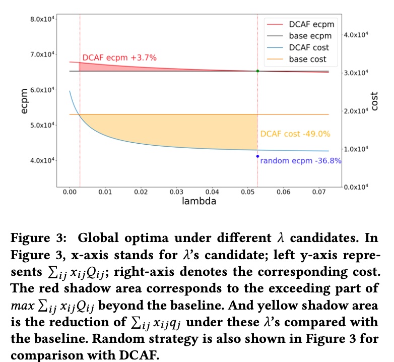
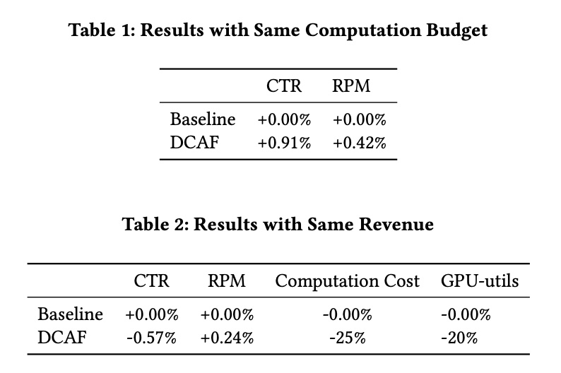
Although offline shows +3.7% eCPM with same cost, -49% machine cost with same eCPM, but after all it’s offline environment, relatively stable, and chosen action won’t affect environment. So online experiment results will generally be discounted, as shown in the paper’s online experiment:
Traffic Value and Computational Cost Modeling
DCAF paper emphasizes allocation strategy but doesn’t say much about traffic value and computational cost modeling, only mentioning \(Q_{ij}\) is estimated through a simple linear model, while \(q_j\) is just candidate count without modeling. But modeling these two variables greatly affects results, especially \(Q_{ij}\).
Note that both traffic value \(Q_{ij}\) and computational cost \(q_j\) are positively correlated with candidate count, and more candidates approach traffic’s maximum value (with controllable error rate), while consuming more computational resources.
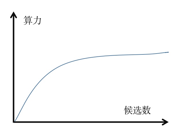
Directly using candidate count as computational cost isn’t very accurate. For example, all candidates only need feature extraction once, this time won’t increase with candidate count. If we plot candidate count on x-axis and computational cost on y-axis, we’ll likely get a curve like \(\log(ax)+b\) (\(a\) and \(b\) are parameters), i.e., marginal computational cost decreases as candidate count increases. Same for \(Q_{ij}\). So we can write both \(Q_{ij}\) and \(q_j\) as \(f(candidate\_count)\) function form.
Meituan’s article describes their improvement on DCAF, Meituan Food Delivery Ad Intelligent Computational Resource Exploration and Practice, including detailed modeling for both parts. Below I’ll describe Meituan’s approach and discuss other possible approaches.
Traffic Value Modeling
If directly modeling \(Q_{ij}\) (e.g., through multi-head approach where each head represents an action), we need to ensure \(Q_{ij}\) monotonically increases with \(j\). We can add regularization term in loss to ensure estimated values are increasing as much as possible, like adding \(ReLU(pred_{j}-pred_{j+1})\) term in loss to keep predictions ordered, but this can’t completely guarantee predictions are ordered.
To address this, Meituan’s approach is estimating entire traffic’s value, then estimating different tier values through each ad’s estimated score (i.e., tier value estimation below). This theoretically can calculate all possible actions, more flexible and lightweight than multi-head approach.
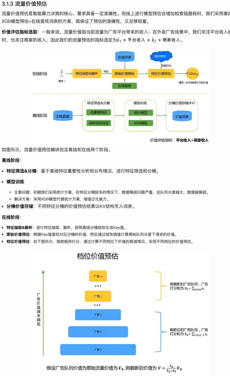
For value estimation, to ensure online efficiency, Meituan uses “offline estimation, online query” method, i.e., offline partitioning traffic through feature bucketing, then estimating each bucket’s traffic value through XGBoost and writing to external KV. Online serving through real-time KV query and interpolation ensures every traffic has an estimate, finally getting \(Q_{ij}\) under different \(j\) through tier value estimation.
Besides this approach, as mentioned earlier, if candidate count is x-axis and computational cost y-axis, we’ll likely get a \(\log(ax)+b\) form curve. We can do simpler inference and solving based on this prior, like directly fitting \(a\) and \(b\) parameters based on posterior data, but need to consider at what granularity - e.g., user granularity, user × ad slot granularity, etc. The core question is what granularity to use. If too fine, data is sparse, may need to use larger granularity. Bayesian methods can also be considered.
Computational Cost Modeling
Meituan’s computational cost modeling is similar to value modeling, both using offline estimation and online query.
Offline feature bucketing first, then modeling relationship between item count and computational cost in each bucket. Each bucket’s modeling uses piecewise linear fitting. Unlike value modeling, there’s no interpolation here (defaulting all traffic can find corresponding bucket?).
Unlike DCAF original paper using item count to measure computational cost, here CPU time is used. Overall approach:
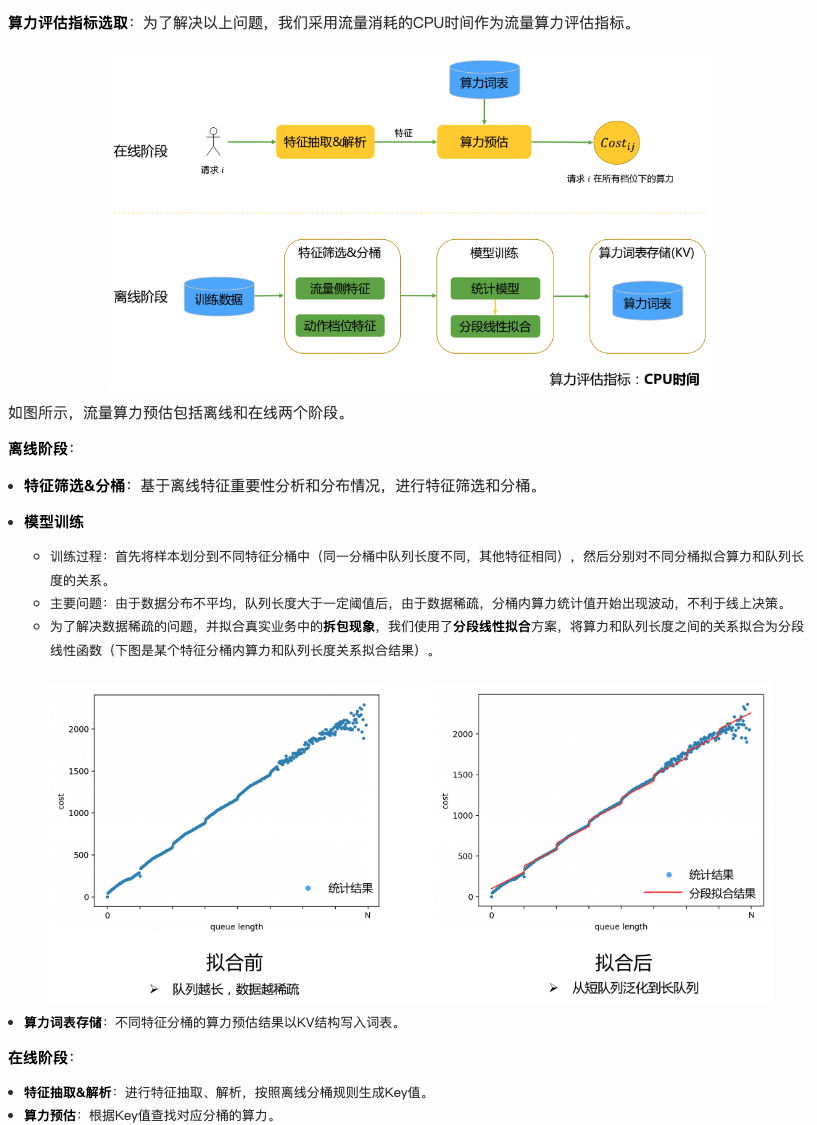
Another approach is similar to using \(\log(ax)+b\) as prior mentioned above, also needing to fit \(a\), \(b\) parameters at specific granularity.
Summary
This article mainly introduces computational resource optimization methods from traffic dimension, summarizing them into drop, cache, and dynamic methods. If we decompose computational resources into “QPS × average request computational cost”, drop discards some low-quality requests, cache reduces average request computational cost through caching. Both methods are straightforward.
Dynamic also tries to reduce average request computational cost, or more accurately, reallocate computational resources to maintain business effectiveness while reducing machine resources, or maintain machine resources while improving business effectiveness. DCAF is a typical work for this approach. DCAF’s problem modeling and solving are worth learning, but traffic value and computational cost modeling is quite rough. Meituan technical team’s article provides good supplementation for this part. This article also proposes ideas for modeling these two variables. Overall, this method has proven effective in both theoretical derivation and industrial practice, worth learning.