Mix-Ranking Between Ads and Organic Content
Mix-ranking is often the final stage in recommendation systems, where natural content (hereafter item) needs to be mixed with marketing content (hereafter ad) to generate the final list pushed to users.
From a Long Term Value (LTV) perspective, this is a trade-off process between LT and V. If ads appear too much, they’ll inevitably squeeze item count and positions, affecting user experience and retention (LT), but correspondingly ad revenue, or Average revenue per user (ARPU) will increase, and vice versa.
So industry practice is to set a user experience constraint and optimize ad efficiency as much as possible within that constraint, i.e., maximizing revenue. This can naturally be modeled as an optimization problem. LinkedIn’s 2020 paper does exactly this: Ads Allocation in Feed via Constrained Optimization.
Intuitively, mix-ranking has 2 sub-problems to solve: (1) How to calculate each item or ad’s value at each position: Since items and ads are ranked separately with different objectives, their final value scales are different. How to bring both scales to a comparable range is a question to discuss. (2) How to allocate to maximize final list value: After confirming item and ad values, how to insert item and ad positions to achieve entire list maximization.
LinkedIn’s paper above focuses on the second problem, with some content also involving the first problem. This article will first describe the paper’s modeling approach, then discuss ideas for calculating item and ad values, and other matters to note in mix-ranking.
Modeling Approach
The paper models the problem as the optimization problem below (single request optimization, not considering inter-request optimization for now):
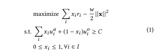
Symbol meanings:
- \(i\): Position index in a request
- \(x_i\): Whether to insert ad at position i
- \(j\): Request index
- \(u_{i}^{o}\): Item’s engagement utility at position i (understandable as content’s inherent value, both item and ad have this)
- \(u_{i}^{a}\): Ad’s engagement utility at position i
- \(r_{i}\): Ad’s revenue utility at position i (understandable as commercial value, items don’t have this)
- \(C\): Global engagement utility threshold. One possible way is setting it as a percentage of maximum possible engagement utility (no ads)
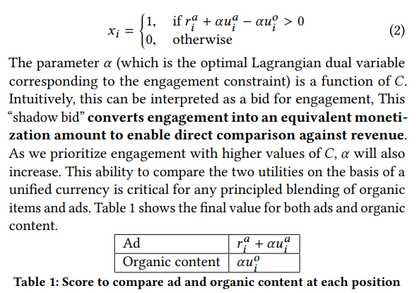
Through dual Lagrangian, we can derive the following solution. \(\alpha\) is the Lagrangian multiplier for the first constraint above. This variable’s physical meaning is a bid - the paper calls it “shadow bid”, functioning to transform engagement utility scale to revenue utility scale. The final value for inserting ad or item at position i is shown in Table 1 below:
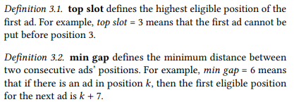
The optimization problem’s constraint above only requires total list engagement utility to be greater than a threshold, but mix-ranking often has hard constraints. The paper mentions: top slot and min gap, representing constraints on first ad position and minimum gap between two ads. Besides these, other common constraints include showtime gap constraint (ad appearance frequency), adload constraint (ad appearance ratio), etc.
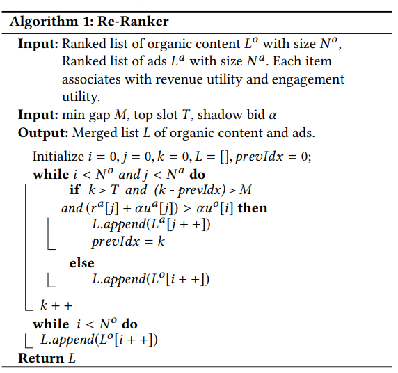
These two constraints aren’t directly in optimization modeling but in the final mix-ranking algorithm. The entire algorithm flow:
Key Modeling Issues Discussion
Although the above modeling is intuitive, there are key issues to solve:
Shadow bid \(\alpha\) Calculation
The paper’s shadow bid is called shadow price in economics, physically meaning marginal benefit from increasing one unit of resource. For more discussion on shadow price, see How to understand shadow price in linear programming?
This shadow price \(\alpha\) is a function of \(C\). The paper mentions three methods to obtain this value:
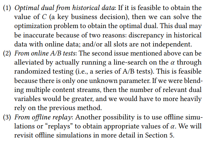
From the figure above, basic idea is: (1) After determining \(C\) value, solve original problem to get \(\alpha\) (2) Determine this parameter through online AB experiments (3) Offline replay (feels the same as the first, since solving original problem also requires replaying historical data, just how much historical data and update frequency)
\(u_{i}^{o}\), \(u_{i}^{a}\) and \(r_{i}\) Calculation
For obtaining these values, the paper doesn’t provide a clear method, only mentioning “\(u_{i}^{a}\), \(u_{i}^{o}\) and \(r_{i}\) are drawn from the same distribution as was the historical data”.
But if we do this, the inevitable problem is historical data will be sparse, making new items or ads have no data, or if we expand the dimension for statistical historical data, this easily leads to worse results with no discriminative power in data. Therefore, we ultimately need to move toward estimation direction.
If we consider actual business, \(u_{i}^{o}\) and \(r_{i}\) are easy to obtain - directly use scores from original item ranking and ad ranking. But how to get \(u_{i}^{a}\)? (Actually \(u_{i}^{o}\) and \(r_{i}\) also have a problem - how to get \(u\) or \(r\) for an item or ad at all positions. This is discussed in position bias section below.)
If we let ads go through recommendation-side model directly, it makes physical sense, but might have 2 problems: (1) ad features might not fully align with item features (2) need to ensure \(u_{i}^{a} \lt u_{i}^{o}\).
The second problem is especially important. If this doesn’t hold, the optimization problem’s final solution will be to show ads whenever possible while satisfying top slot and min gap constraints, which is obviously unreasonable. How to guarantee this? I haven’t thought of a good method. For example, using multi-head in recommendation model with one head estimating items and one head estimating ads, trying to ensure item head > ad head through regularization, but can’t make strict guarantee.
position bias
This issue was mentioned in the \(u_{i}^{o}\), \(u_{i}^{a}\) and \(r_{i}\) discussion above.
If we don’t consider position information when calculating \(u_{i}^{o}\), \(u_{i}^{a}\) and \(r_{i}\), it’s inevitably biased because CTR, CVR etc. naturally differ at different positions.
The paper mentions one method, also commonly used in practice: training phase uses actual position, serving phase uses unified position, while keeping a mapping table mapping different positions to discount relative to unified position used in serving. The mapping table can be obtained through posterior data statistics. Final estimated value multiplied by this discount gives estimated value at different positions.
The drawback is this mapping table needs frequent updating. A better approach is putting this table into the model so it learns this variation during training, estimating scores at all positions simultaneously during estimation phase.
gap effect
For recommendation, order accuracy is often sufficient, but ads involve actual billing, requiring sufficiently accurate CTR, CVR estimation to avoid inaccurate billing causing advertiser complaints etc.
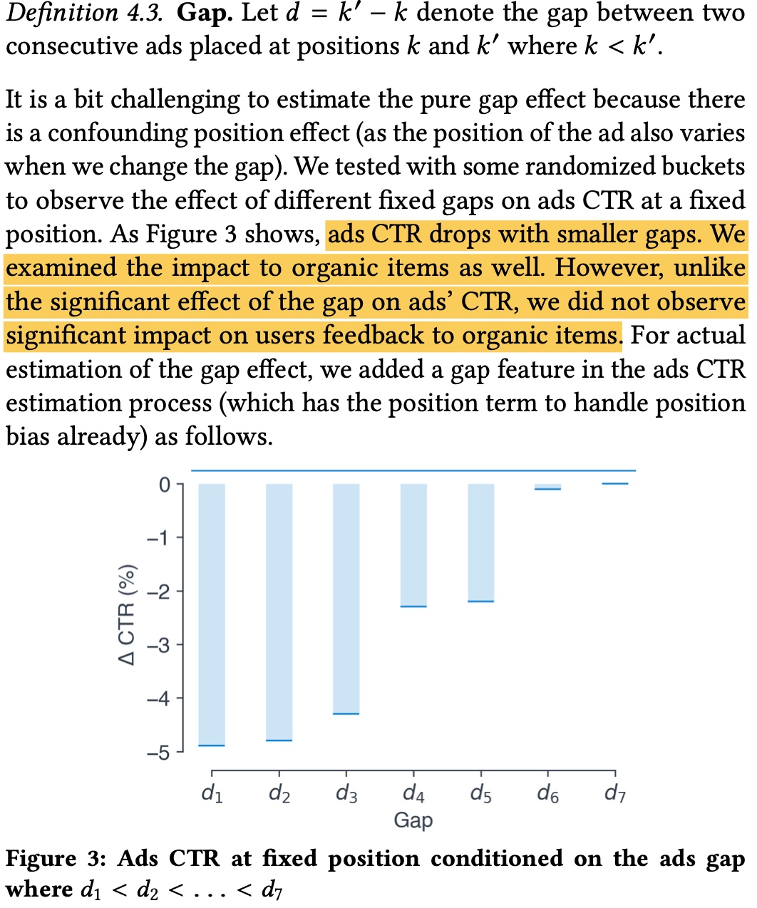
Besides position bias above affecting CTR accuracy, the gap size between two ads also affects ad CTR etc. As shown below, if ad gap is too small, ad click rate will be low, but items don’t have this problem. Fundamentally because ad density is too high, even with min-gap hard rules mentioned earlier.
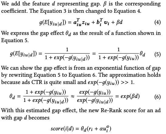
The paper’s approach is adding a gap feature to capture this information. The paper derives as shown below, final effective form is like position_discount, equivalent to multiplying original CTR by gap_discount. \(g\) in the figure is Logit function, \(y_{ij}\) indicates whether click occurred (can further parameterize \(\beta\) to make it personalized).
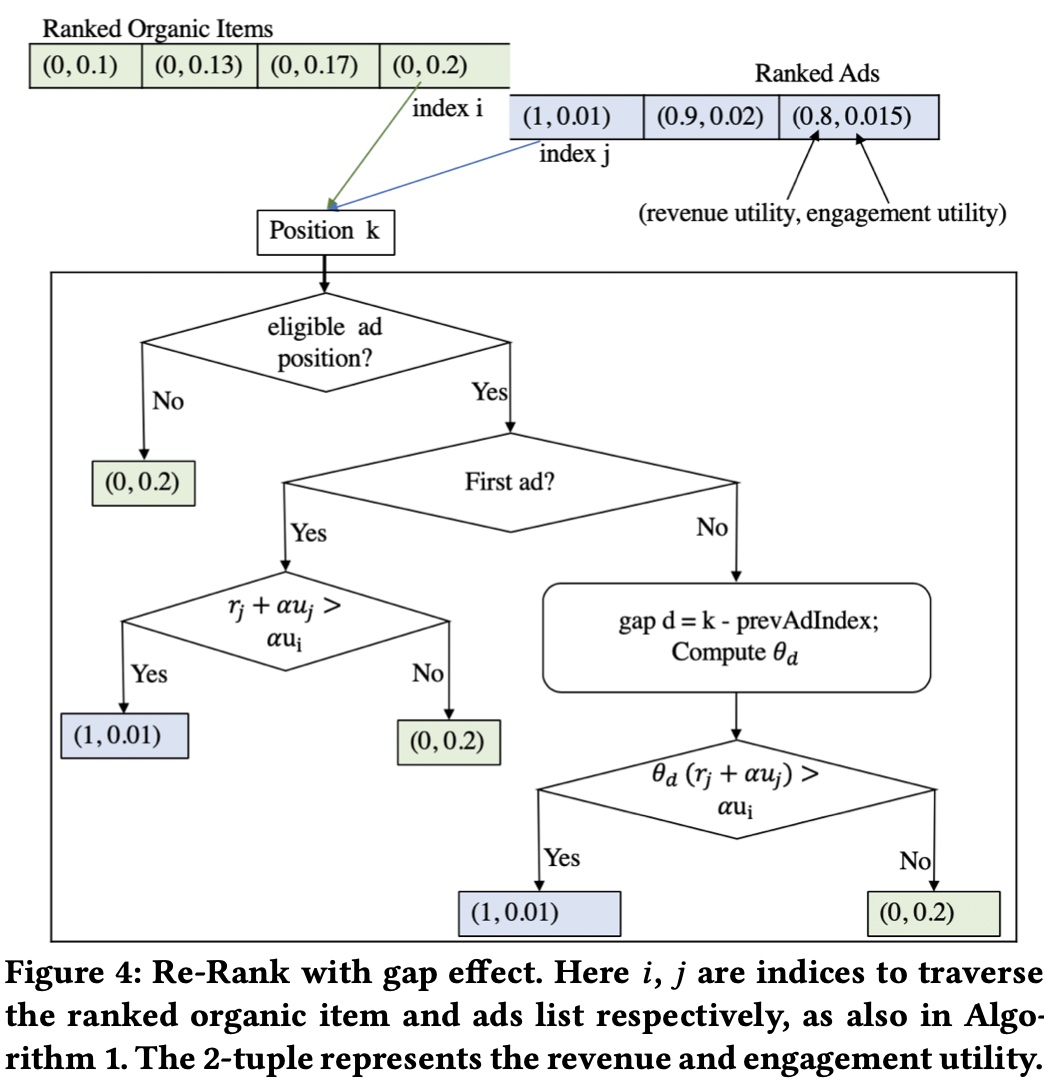
If we add gap effect in the mix-ranking algorithm above, the flow:
Another Approach for Item and Ad Value Measurement
The paper considers item value as engagement utility, ad value as engagement utility + revenue utility.
As mentioned above, obtaining ad’s engagement utility is difficult. Therefore, we can consider another approach for measuring item and ad value.
Since ads involve billing, ad value is easy to measure, generally using eCPM = bid × ctr × cvr (for discussion simplicity, omitting hidden_cost here). So naturally: can we assign a bid to each item too, so we can calculate an eCPM-like metric for items, comparable to ads?
The immediate question is: what does item-side bid mean? Ad-side bid has clear physical meaning: money advertiser is willing to pay for a conversion (also modified by adjustment strategy on original advertiser bid). But there’s no advertiser role on item side, so who provides this bid?
The most intuitive method is setting a global fixed bid for item side based on the scale difference between ad and item estimated values, but this is obviously not optimal. And this bid’s scale also needs timely monitoring and updating because both sides’ estimated value scales will change with iteration.
From another perspective, ads express advertiser needs, targeting more user conversions. Items express platform needs, targeting bringing more users and retention time to the platform. Longer retention time also means more traffic available for platform monetization, or user metrics are actually linked to platform long-term revenue. Therefore, we can measure the relationship between user metrics and platform revenue at overall level. Taking stay_duration as example, we can bucket stay_duration and measure its correlation with platform long-term revenue indicators, building a function \(f\) such that \(bid = f(stay\_duration)\). Of course, the variable doesn’t have to be stay_duration - it can consider dislike, active, and various signals. The key is quantitatively linking user retention and activity info with platform long-term revenue, then deriving an item-side bid based on this revenue.
For ads, when mixed ranking with items, the benefit from placing ad at position \(k\) among items isn’t just the ad’s eCPM, but can further consider loss to overall items from ad insertion (VCG billing idea), i.e., mix-ranking ad value can be considered as “ad benefit - item displacement loss”. This way, if insertion position causes large item displacement loss, overall ad value decreases, avoiding item squeeze.
Are Hard Rules Optimal?
As mentioned earlier, mix-ranking has various hard rules like ad first position, min_gap between ads, show_time gap, etc. From technical perspective, such discrete hard rules obviously aren’t optimal, greatly limiting algorithm search space. From business perspective, such hard rules are often determined in early business development. As business develops, whether current rules are reasonable also needs re-evaluation.
For example, using same hard rules for ad-sensitive and ad-insensitive users isn’t optimal. Same ad frequency has lower conversion rate for sensitive users while also having larger impact on user retention (compared to insensitive users). If we show more ads to ad-insensitive users while reducing ads for sensitive users, balancing total ad count, final engagement utility and revenue utility would theoretically be better.
In implementation, we generally need to set rules and calculation methods to calculate utility for all possible hard rule situations, then add to list’s total value.
This actually involves an optimization direction in recommendation or ad systems - personalization. Generally, any overall strategy with same hyperparameters or strategy for all users has personalization potential.
Of course, in this process we need to note personalization also has limits. For mix-ranking, we need experience protection for insensitive users, can’t keep exploiting them.
Summary
This article starts from LinkedIn’s paper, introducing problems mix-ranking needs to solve and a modeling approach. The paper’s modeling isn’t complex - the key is obtaining various utilities in modeling. The paper doesn’t describe this in detail, possibly because it’s tightly coupled with specific business. Therefore, this article later discusses a possible approach for calculating item and ad values: calculating a bid for items while considering ad insertion’s impact on items.
Additionally, the paper mentions position bias, gap effect, and other common issues in mix-ranking. This article discusses the paper’s proposed methods and some industry approaches.
Finally, it explores a relatively open question - hard rules in mix-ranking. Hard rules are generally red lines, but from technical perspective definitely not optimal. Whether hard rules are reasonable, and how to soften hard rules from business and technical perspectives to get benefits in both engagement utility and revenue utility, might be worth discussing.