Loss Functions for Regression Tasks

In search/recommendation/advertising related businesses, besides common binary classification tasks like CTR and CVR, there are a series of regression tasks estimating stay_duration, LTV, ECPM, GMV, etc.

CTR/CVR binary classification tasks commonly use cross-entropy loss, with the basic assumption that events follow Bernoulli distribution, ultimately learning the proportion of positive samples. But regression tasks have many optional loss functions, like MSE, MAE, Huber loss, log-normal, weighted logistics regression, softmax, etc.

Each loss function has its assumptions and applicable scope. If the real label distribution differs significantly from assumptions, results can be poor. Therefore, this article focuses on the derivation process and assumptions of these common losses.

MSE/MAE/Huber

These three losses are the most intuitive and common losses for regression tasks. The first two both assume errors follow specific distributions, then derive the final loss form through MLE. Huber is a hybrid version of the first two losses.

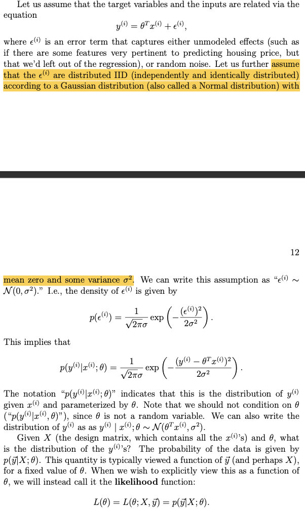
MSE assumes the error between predicted and actual values follows standard Gaussian distribution, then writes the error likelihood function and derives the final loss form through MLE. The derivation process is shown below (from CS229 textbook):

Based on errors following Gaussian distribution with mean 0, we can write the likelihood function:

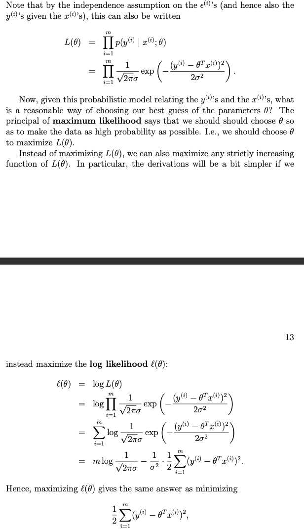
Then based on IID assumption and MLE, we can write the final loss function:

MAE derivation is similar to MSE, just assuming errors follow Laplace distribution. Replace Gaussian distribution in the derivation above with Laplace probability density function to get the final MAE loss form.

From the loss function form, we can intuitively see that for the \(i\)-th sample:

• MSE backpropagation gradient size is \(-(y^{(i)} - \theta^{T}x^{(i)})x^{(i)}\)
• MAE backpropagation gradient is \(- \frac{y^{(i)} - \theta^{T}x^{(i)}}{|y^{(i)} - \theta^{T}x^{(i)}|}x^{(i)}\) (actually ±\(x^{(i)}\), absolute value derivative reference Derivative of Absolute Value)

From the backpropagated gradients, MSE is easily affected by outliers. For example, if there’s an outlier sample with very large label, the \(y^{(i)} - \theta^{T}x^{(i)}\) value will also be very large when computing gradient, easily biasing the sample. MAE is less affected by this.

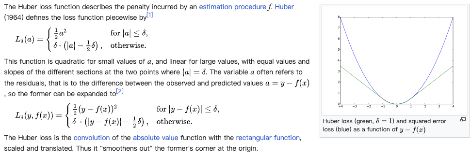
So Huber Loss considers this, using MSE for samples with small labels and MAE for samples with large labels. The entire loss form:

ZILN(Log-normal)

This is a loss proposed in a Google paper for estimating LTV, A Deep Probabilistic Model for Customer Lifetime Value Prediction.

Real-world data is often long-tailed and sparse. Taking the LTV task in the paper as example, there are many 0 values, also extreme high values. Below shows the LTV distribution in the paper (LTV here means value generated after first purchase, 0 means many customers only purchased once):

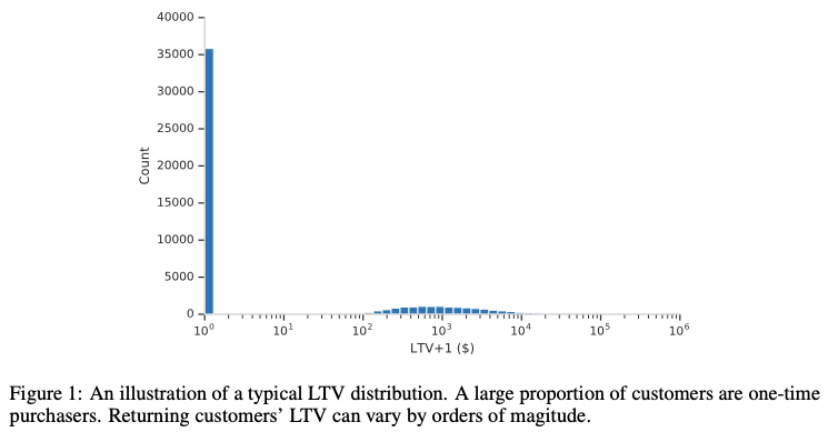
The paper mentions directly using MSE has the following problems, which are also the MSE issues mentioned above:

MSE loss does not accommodate the significant fraction of zero value LTV from one-time purchasers and can be sensitive to extremely large LTV’s from top spenders

So the paper proposes ZILN (Zero-Inflated LogNormal) loss, with form below (note \(x\) is label):

\[\begin{align} L_{ZILN}(x;p,\mu,\sigma)= -\mathbf{1}_{x=0} \log(1-p) - \mathbf{1}_{x>0}(\log p - L_{Lognormal}(x;\mu,\sigma)) \end{align}\]

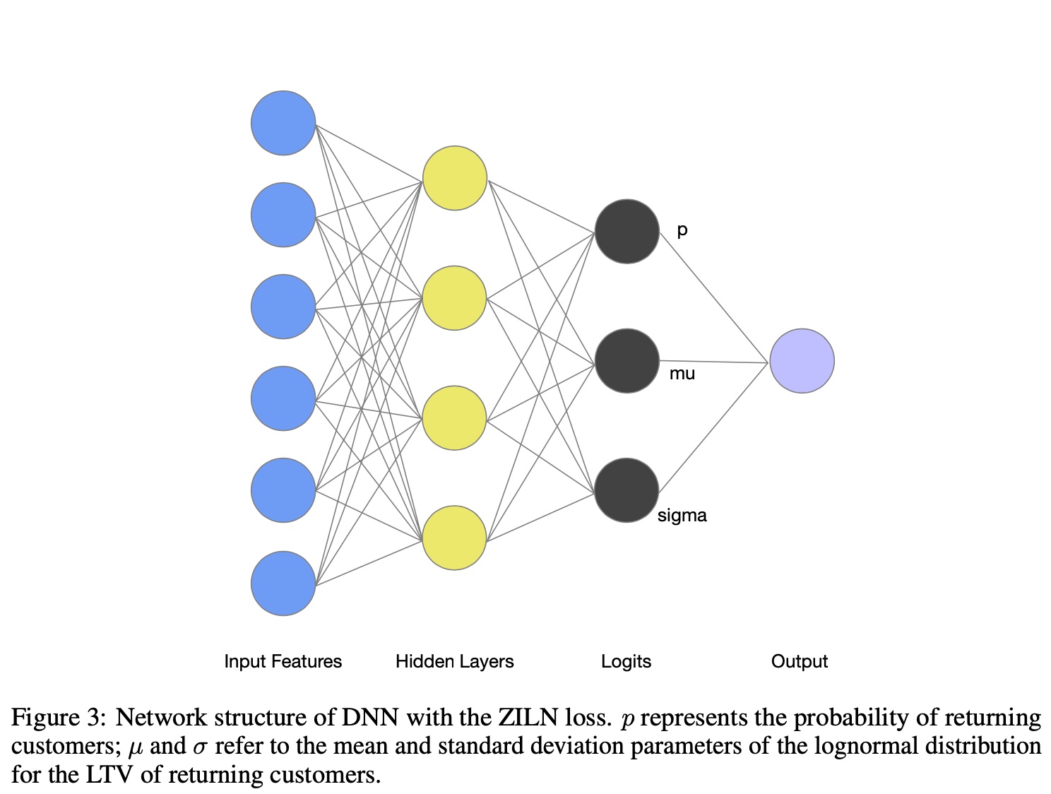
This loss actually has 2 terms, corresponding to modeling LTV as 2 tasks in the paper. One estimates purchase probability (\(p\) in formula above), the other estimates purchase amount. The first task uses common classification cross-entropy loss. This idea is quite common - introducing intermediate signal modeling often makes overall results better, like modeling CTR and CVR separately, or modeling send2click as send2show and show2click separately.

Here I focus on the second task, the loss for estimating amount \(L_{Lognormal}(x;\mu,\sigma)\). This loss form:

\[\begin{align} L_{Lognormal}(x;\mu,\sigma)=\log (x \sigma \sqrt{2\pi})+\frac{(\log x - \mu)^2}{2 \sigma^2} \end{align}\]

This is actually the log-normal distribution probability density function with log transformation applied. The implicit assumption is LTV follows log-normal distribution, while parameterizing \(\mu\) and \(\sigma\) (using a DNN to estimate them, note \(x\) is still label).

The final model outputs 3 estimates \(p\), \(\mu\) and \(\sigma\):

Log-normal form derivation can reference the wiki link above or Log-Normal Distribution. Simply, when a variable \(X\) follows log-normal distribution, its logarithm \(\ln X\) follows normal distribution, and vice versa.

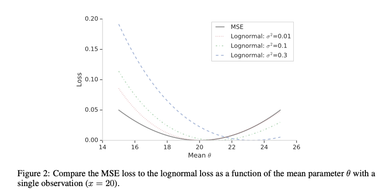
Compared to MSE, log-normal doesn’t produce very large loss even when estimates are very large, somewhat alleviating the MSE problems mentioned earlier.

Weighted Logistics Regression

This loss was applied in Google’s famous 2016 paper to estimate user watch duration, Deep Neural Networks for YouTube Recommendations. In practice, many variants and implementations based on this idea exist, essentially converting regression tasks to classification tasks.

From the name, we can guess the loss form - reweighting a classification loss. Specifically, using cross-entropy loss, then for positive samples (clicked samples in modeling watch duration), use the actual watch duration \(T\) for reweighting, negative samples unchanged.

After reweighting, this changes the positive-negative sample ratio in original samples (treating watched as positive samples, not watched/clicked as negative samples). We know cross-entropy ultimately estimates the probability as the proportion of positive samples. After reweighting, a sample with label \(T\) is equivalent to \(T\) positive samples in the classification task.

So the overall sample positive ratio becomes \(\frac{\sum_{i=1}^k T_{i}}{N + \sum_{i=1}^k T_{i} -k}\), where \(N\) is total sample count, \(T_i\) is each positive sample’s watch duration, \(k\) is positive sample count (this derivation differs from the paper’s but has same principle and result, more intuitive).

From logistics regression estimating positive sample proportion:

\[\begin{align} \frac{1}{1+e^{-logit}}=\frac{\sum_{i=1}^k T_{i}}{N + \sum_{i=1}^k T_{i} -k} \end{align}\]

Since positive samples are often very sparse, the paper omits \(k\). Let \(P=\sum_{i=1}^k T_{i}\), then:

\[\begin{align} \frac{1}{1+e^{-logit}}=\frac{P}{N + P} \end{align}\]

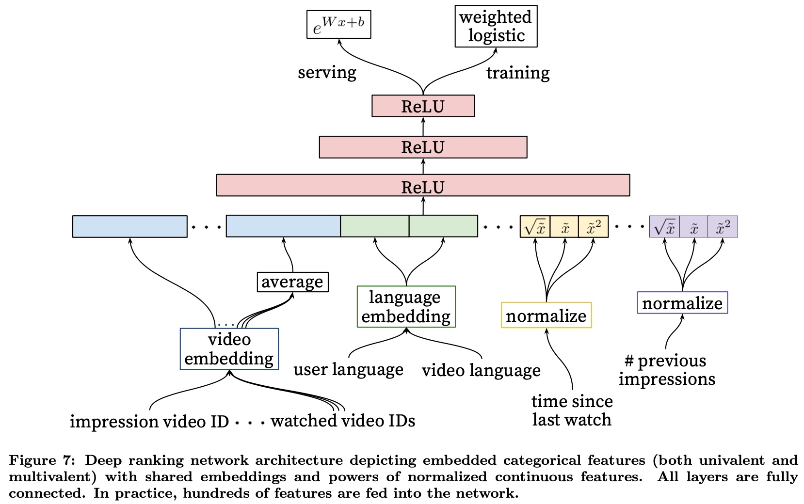
Left side numerator and denominator both multiplied by \(e^{logit}\), right side both divided by \(N\), we can derive \(\frac{P}{N} = e^{logit}\). Since \(P\) is summed, averaged per sample, serving time estimated duration is \(e^{logit}\).

So training uses cross-entropy loss with positive sample reweighting, and serving time after getting logit, take \(e^{logit}\) as final estimate. The paper’s figure shows this process well:

The above derivation omitted original positive sample count \(k\). Strictly speaking, this causes biased estimates. The simplest fix is treating a sample with label \(T\) as \(T\) positive samples and 1 negative sample. Compared to original approach, this adds one negative sample per original positive sample.

Then the original formula becomes, where first \(k\) in right side denominator is original positive sample count, second \(k\) is added negative sample count:

\[\begin{align} \frac{1}{1+e^{-logit}}=\frac{\sum_{i=1}^k T_{i}}{N + \sum_{i=1}^k T_{i} - k + k} \end{align}\]

Returning to this loss’s assumption, cross-entropy assumes labels follow Bernoulli distribution with parameter \(p\), then MLE derives cross-entropy form.

After above reweighting on cross-entropy, it’s equivalent to assuming labels follow geometric distribution with parameter \(p\) (not very rigorous, since \(p\) here is failure probability). The reweight value (label \(T\)) is the value extracted to front after geometric distribution PDF takes log, meaning consecutive failures \(T\) times (opposite physical meaning from original geometric distribution).

Bucketing With Softmax

In regression, another approach is bucketing + softmax. The idea is intuitive - bucket the label’s value range, then assign each sample to a bucket based on its label. Training becomes a multi-classification problem using softmax loss.

Serving uses softmax estimated probability distribution to compute weighted sum over buckets. With \(n\) buckets, \(p_i\) as each bucket’s probability, \(v_i\) as each bucket’s value (usually bucket midpoint):

\[\begin{align} pred = \sum_{i=1}^{n} p_i v_i \end{align}\]

This method’s key is how to bucket, including number and size of buckets. Both variables significantly affect final results. Too many buckets leads to sparse samples per bucket, too few leads to no discriminative power in estimates.

Common approach is manual bucketing based on label’s posterior distribution. Since real data is often long-tailed (more small label samples), use more buckets with smaller intervals for smaller labels. The goal is balanced samples per bucket. But bucket count and size are hyperparameters needing tuning.

Besides using bucket mean directly, can also apply losses like MSE per bucket. This becomes partition-wise multi-task modeling or stacking in ensemble.

Another common operation in this type of method is label smoothing. The motivation is the original approach loses ordinal relationship between labels. For example, assigning a label=50 sample to [0,10] bucket vs [51,100] bucket has no difference in loss. So a natural idea is making original one-hot label smoother.

Specifically, transform label during training to make it similar to Gaussian or Laplace distribution form. For example, original label [0, 0, 0, 0, 1, 0, 0, 0] after smoothing becomes [0, 0, 0.01, 0.03, 0.9, 0.03, 0.02, 0.01]. The transformation method is also a hyperparameter.

Overall, this method involves considerable prior knowledge - how to bucket, how to choose label smoothing function. But avoids prior assumptions about label distribution, theoretically applicable to any regression task. However, needs periodic review to prevent prior assumptions from becoming invalid when overall data changes.

Ordinal Regression

Ordinal regression is suitable for scenarios caring about different values’ order but not absolute values. Quoting wiki:

variable whose value exists on an arbitrary scale where only the relative ordering between different values is significant. It can be considered an intermediate problem between regression and classification

Common tasks like rating, e.g., rating image/video obscenity level. Not using classification directly because of the label smoothing issue mentioned above for bucketing - no difference between buckets.

Specific loss form is also derived through MLE, but unlike formulas above based on PDF (Probability Density Function) for MLE derivation, here using CDF (Cumulative Distribution Function). Derivation shown below. From derivation, the assumption is also “error \(\epsilon\) follows standard normal distribution”, same as MSE.

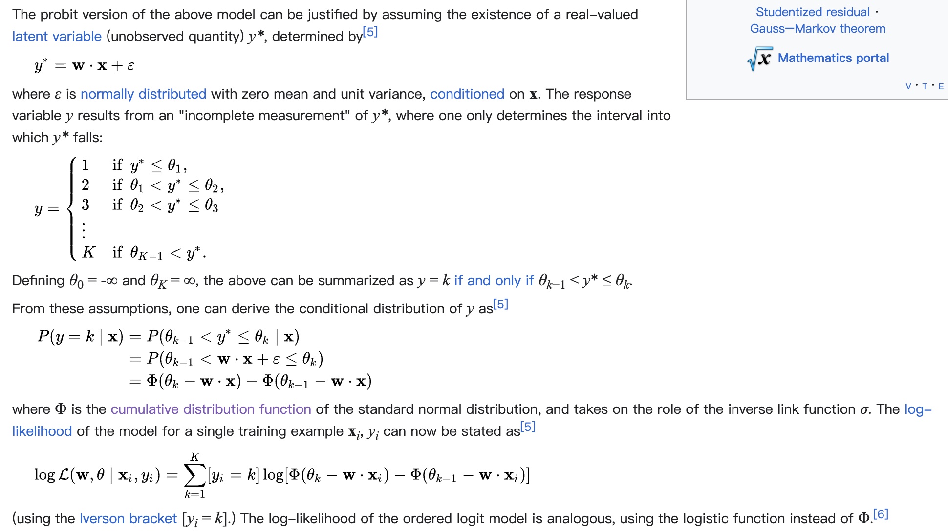
The thresholds \(\theta\) distinguishing samples in different intervals are also parameters learned through training. Final serving output depends on \(\theta\) and specific estimates. This article provides an implementation reference: Ordinal Regression for Handling Grading Problems.

Notably, for rating tasks, labels are clear. But for general regression tasks, there’s still a process of partitioning intervals or assigning rating per label. Like softmax methods above, this is also a hyperparameter.

Summary

This article mainly describes common loss functions in regression tasks. Each loss function has different assumptions with different applicability.

MSE, MAE, Huber Loss are common and intuitive regression losses, assuming predicted-actual difference follows normal or Laplace distribution.

Log-normal loss directly assumes labels follow log-normal distribution, deriving through MLE to solve for log-normal PDF’s mean \(\mu\) and variance \(\sigma\) parameters (binary classification’s cross-entropy uses same principle, just different distribution - Bernoulli, with parameter \(p\) for event probability).

Besides direct estimation, there are methods converting to classification for indirect estimation, mainly 2 approaches: (1) Weighted Logistics regression (2) Bucketing With Softmax.

Weighted Logistics regression treats a sample with label \(T\) as \(T\) positive samples (and one negative sample), statistically ensuring unbiased estimates. Widely applied in practice, with underlying assumption that labels follow geometric distribution.

Bucketing With Softmax uses prior bucketing of labels, then estimates probability distribution of labels falling in each bucket through softmax, finally computing probability-weighted sum over buckets for final estimate. This method’s advantage is no distribution assumptions, theoretically applicable to all distributions. But effectiveness heavily depends on bucket count and size. Also involves improvement techniques like label smoothing, stacking.

Ordinal Regression is a regression loss caring about order but not absolute value error. Same assumption as MSE but uses CDF instead of PDF for loss derivation, learning thresholds for different levels through training. Commonly used in rating tasks. For more general regression tasks, still relies on manual interval partitioning for different ratings.