Adload-Constrained Mix-Ranking Value Maximization
The previous mix-ranking article mainly introduced the basic approach from “Ads Allocation in Feed via Constrained Optimization” and extended the discussion to open problems in mix-ranking. That paper solves request-level insertion rules but doesn’t consider practical constraints like adload, i.e., the proportion of ads shown is limited.
When considering adload constraints, we can’t just compare values within requests; we need to maximize value across requests or at the session level. For example, showing more ads on high-value requests and fewer or no ads on low-value requests to maximize revenue under adload constraints. This paper “Hierarchically Constrained Adaptive Ad Exposure in Feeds” provides a solution approach. The paper’s overall approach still uses beam search and the generator+evaluator mix-ranking paradigm, but incorporates overall constraints into the online solving process. Compared to conventional approaches that control adload independently from mix-ranking, this is a better approach worth reading~
Problem Modeling
Definition
The paper defines the overall problem as follows:
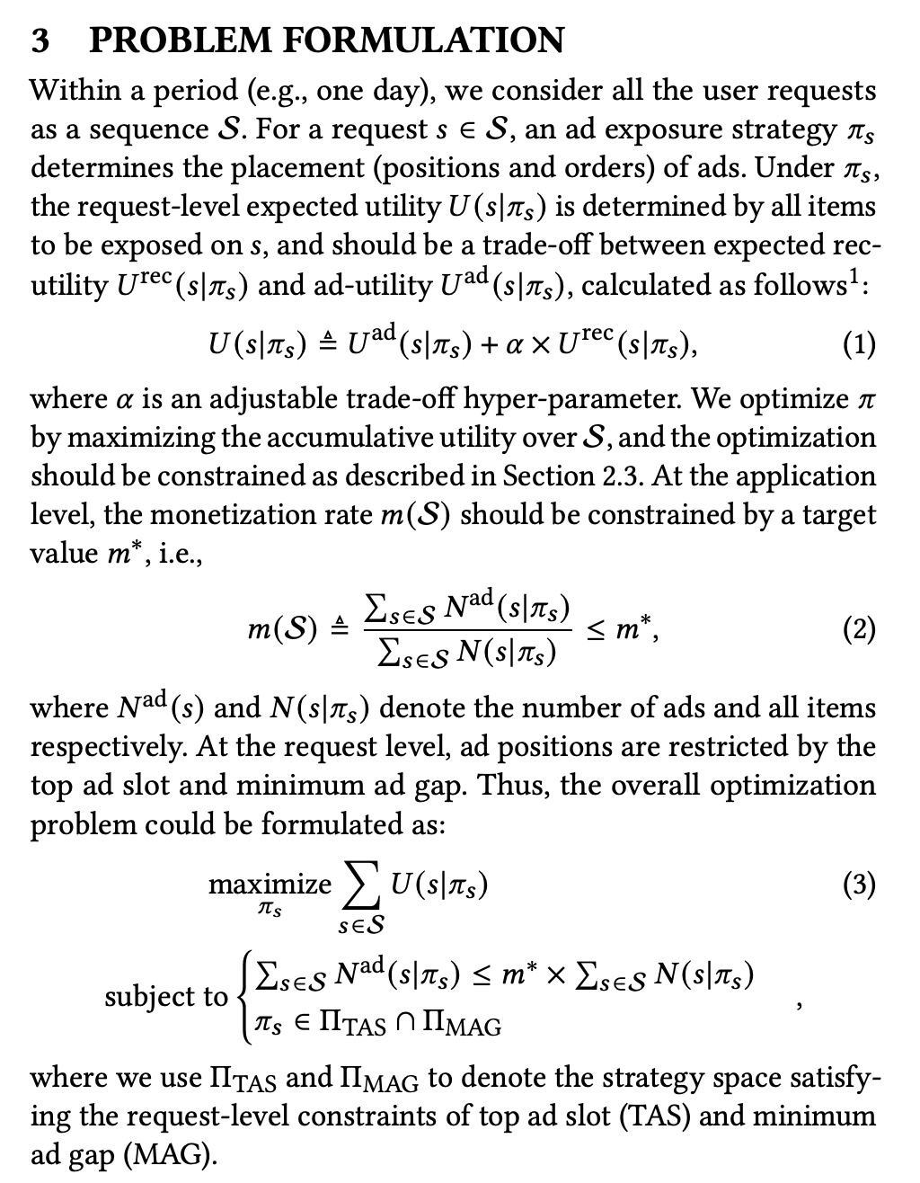
Two points worth noting:
- Value Measurement
Value measurement or scale alignment is an unavoidable problem in the mix-ranking stage. The paper uses a monetization hyperparameter \(\alpha\) to align user value \(U^{rec}(s|\pi_s)\) for recommended candidates and commercial value \(U^{ad}(s|\pi_s)\) for ads.
This is a common industry practice. The reason is that commercial value (ecpm) has relatively clear physical meaning and doesn’t fluctuate easily (since bid is basically stable, and CTR/CVR predictions have accuracy requirements). In contrast, recommendation often only cares about ranking, not absolute values. This can cause issues when recommendation scores fluctuate, potentially leading to accumulation. So stability measures are often applied to recommendation scores, like capping outliers and normalization.
- Application Level Modeling
As mentioned in the background, the previous paper mainly modeled request-level value maximization but didn’t consider adload constraints (the \(m^*\) in the figure below). Here, the modeling considers all requests in a session together.
Modeling
Although the problem definition is simple, directly solving for \(\pi\) is difficult. So we need to transform the problem into a mathematically solvable form. The specific method splits the overall strategy into two parts: application-level strategy \(x\) and request-level strategy \(\pi\). \(x\) decides whether to show ads in this request, while \(\pi\) decides how many ads to show in this request. Besides these symbols, the paper’s notation is defined below:
![]()
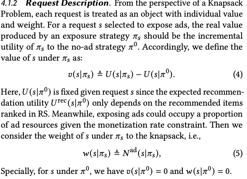
At the request level, value \(v\) (\(\pi_0\) means no ads) and ad count \(w\) are defined as follows. The paper doesn’t clearly explain how \(v\) is calculated. At first glance at formula (4), \(v\) appears to be the sum of ad values, most intuitively \(\sum ecpm\) of pure ad candidates. But this is incomplete: first, it only considers commercial value; second, the impact of ad insertion on recommended content isn’t considered.
The actual calculation should be: value of list with both recommended content and ads - value with only recommended content. This means in beam search, when calculating each list’s value, we need to calculate two values: \(U(s|\pi_s)\) with ads and \(U(s|\pi^0)\) without ads. Additionally, the paper doesn’t give specific calculation methods for \(U(s|\pi_s)\) and \(U(s|\pi^0)\); actual calculation should consider position decay, i.e., multiply by position_discount.
Maximizing value under adload constraints is essentially a classic 0-1 knapsack problem, where adload is the knapsack capacity and we maximize the value of requests showing ads. Based on the symbols defined above, the optimization problem is defined below, where \(x_s\) is whether to show ads in a request:
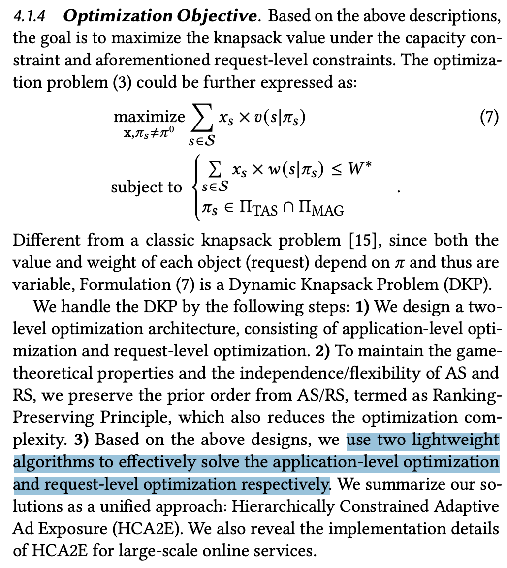
Unlike traditional knapsack algorithms, item values dynamically change as determined by request-level strategy \(\pi_s\). Therefore, the paper designs a two-level algorithm: application level and request level.
Problem Solving
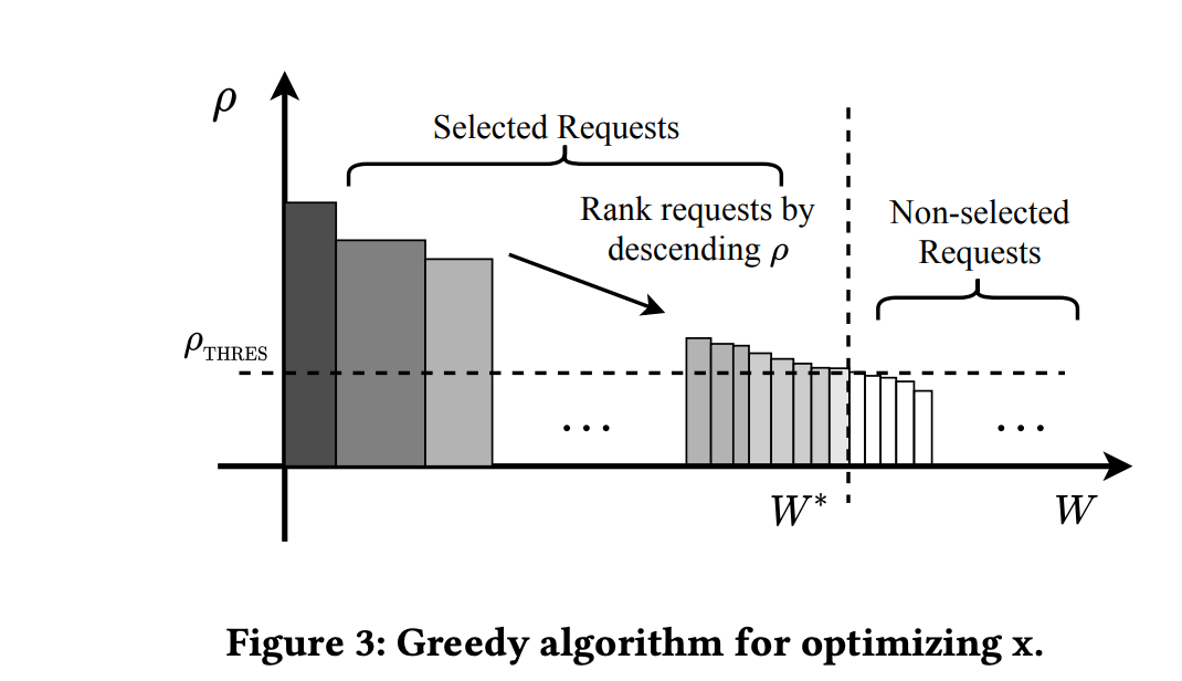
Application Level
Here we use a greedy algorithm to solve the application-level problem, deciding whether to show ads in the current request (note: greedy algorithms are not optimal for knapsack problems but are lightweight enough). The approach is to calculate \(\rho = v/w\) based on the defined \(v\) and \(w\) (can be understood as marginal value of ads), sort by \(\rho\), then find a threshold under adload constraints. Online serving only shows ads for requests above this threshold, as shown below:
Request Level
Request level decides the specific ad strategy \(\pi_s\).
Assume the ad strategy changes from \(\pi_1\) to \(\pi_2\), causing changes in this request’s \(v\) and \(w\) (denoted as \(\Delta v^{+}\) and \(\Delta w_s\)). Since \(w\) changes, other requests will show more or fewer ads, affecting application-level value.
As shown below, value increases by \(\Delta v^+\) within this request, but value decreases by \(\Delta v^-\) in other requests (approximate value using the threshold found above; may not hold in extreme cases). Only when the sum is greater than 0 is this strategy effective.
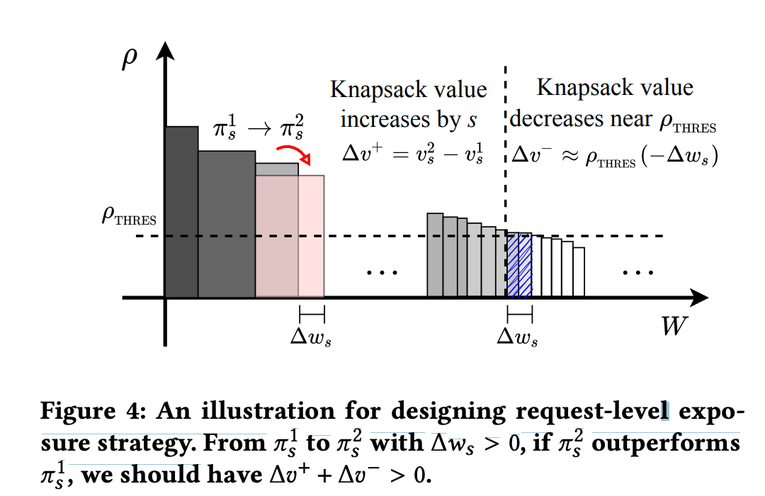
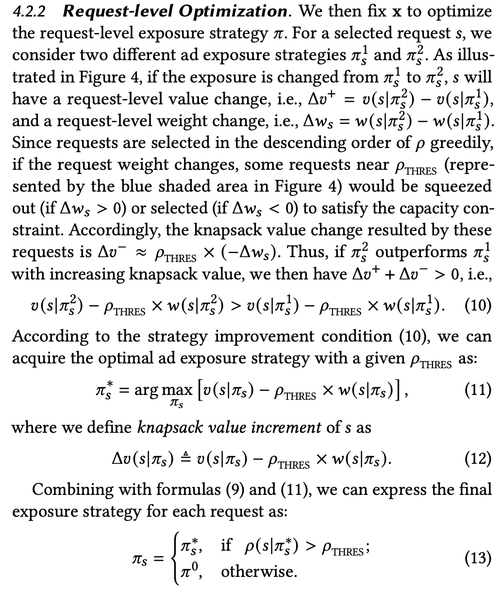
If we expand \(\Delta v^{+} + \Delta v^{-} > 0\), we get formula (10) below. From formula (10), the optimal \(\pi_s\) should maximize \(v(s|\pi_s) - \rho_{thres} * w(s|\pi_s)\), i.e., formula (11):
This is a critical step, transforming a cross-request optimization into one solvable within the current request, since both \(v(s|\pi_s)\) and \(\rho_{thres} * w(s|\pi_s)\) can be computed from the current request.
Order Preservation Problem
Another frequently discussed problem in mix-ranking is whether to preserve the order of input queues. That is, whether the recommended queue and ad queue maintain internal order after mix-ranking. For example, if the ad queue [A1,A2,A3] maintains internal order after mix-ranking, the overall queue would look like […A1…A2…A3…].
Intuitively, order preservation has two important meanings: (1) Not affecting ranking iteration, i.e., ranking AUC metric iteration remains valid; changing ranking order in mix-ranking can make ranking AUC unreadable (2) For ad charging, ads must be in sorted_ecpm descending order, otherwise charging has issues.
The paper approaches this from auction mechanism design, emphasizing the importance of order preservation through Incentive Compatibility (IC) and Individual Rationality (IR).
IC is the commonly mentioned incentive compatibility. Specifically, a mechanism is incentive compatible if and only if when each participant truthfully expresses their preferences, they get higher utility than the marginal, meaning the mechanism encourages participants to express true value expectations. In ads, this means bidding truthfully. IR literally means “individual rationality,” meaning each participant’s utility from participating in the auction is not lower than not participating, i.e., participating doesn’t make them worse off. The paper states:
Formally, if every participant advertiser bids truthfully (i.e., bids the maximum willing-to-pay price), IR will guarantee their non-negative profits, and IC can further ensure that they earn the best outcomes
Why is this related to order preservation? As mentioned above, once order is broken, the charged amount changes, which breaks IC and IR mentioned above. For stricter theory, see Myerson–Satterthwaite theorem, not elaborated here.
But can mix-ranking change ranking order? Since mix-ranking has context information that ranking can’t perceive (like surrounding recommended content, position, etc.), it’s possible to re-estimate CTR/CVR in mix-ranking based on a context model (equivalent to making CTR/CVR predictions more accurate). This case might change order, but it also changes ecpm, ensuring ecpm is decreasing, not violating the problems mentioned above. This is the only reasonable way the author thinks order can be changed in mix-ranking (but this creates a circular dependency: if order changes, context changes, CTR/CVR need re-estimation).
Mix-Ranking Algorithm
The overall algorithm is based on beam search framework, as shown below. The exposure template below refers to candidate lists searched by beam search.
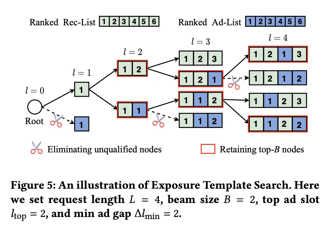
The overall algorithm is shown below. Lines 6 and 9’s formula 14 is essentially formula 12 above, finding the candidate list maximizing \(v(s|\pi_s) - \rho_{thres} * w(s|\pi_s)\). Line 12 prunes candidates violating red-line constraints (like mingap), reducing computational complexity. Lines 13-14 select the top \(B\) candidate lists by value for next search step, standard beam-search.
![]()
Among candidates from beam search, the final decision whether to insert ads is based on the value threshold \(\rho_{thres}\) found at application level, as shown below:
![]()
A noteworthy issue is \(\rho_{thres}\) update frequency. If updating daily, i.e., calculating a \(\rho_{thres}\) from past n days and keeping it constant today, current traffic fluctuations can cause adload to exceed or underfill. One solution is increasing update frequency with more real-time data (e.g., hourly updates using past n hours of data). Another solution is adding a pacer on top of the output \(\rho_{thres}\) to control real-time adload - raise threshold when adload exceeds, lower when under (similar to common sorted_ecpm threshold control for adload).
Summary
Within the widely used “list value evaluation + beam-search” mix-ranking framework, the paper considers maximizing overall value (organic + ads) under adload constraints. Compared to more common approaches that only consider ad-side information for adload control (like adjusting ecpm threshold), this has innovation. Besides adload constraints, other constraints can also use this modeling and solving approach to integrate into the overall mix-ranking algorithm.