Recently I’ve been researching search relevance, a problem with search-specific characteristics. Search relevance means content shown to users must satisfy certain association with user-input query. For example, searching “KFC” shouldn’t show “McDonald’s” content.

Unlike feed scenarios where users have no content expectations, feed recommendation algorithms can exploit based on user browsing history, recent hot content, etc., or explore new interests. But in search scenarios, user-initiated queries have strong intent. Returned content must match this expectation, otherwise the search is invalid, causing search retention (LT) loss. From user perspective, if platform search works well, they should find desired content on first page, leading to much lower search browsing depth per PV than feed.

Scenario differences lead to different optimization objectives for search vs feed. For example, duration isn’t the most important metric for search LT measurement. From ranking perspective, added relevance constraints mean limited candidates for ranking under specific query (compared to feed), while ranking formulas often add relevance factors to achieve relevance objectives, interfering with maximizing original objectives (like revenue for ads).

Relevance constraints in ranking are why many effective feed ranking iterations are suboptimal or ineffective in search. For example, the phenomenon mentioned in Why are there few search system tech articles but many recommendation system articles? - an important reason is given query, insufficient relevance candidates limit ranking search space, while ranking’s benefit should have increasing marginal efficiency as candidate count increases.

This article discusses solution approaches for search relevance. Roughly, relevance involves two parts: relevance modeling, and the mechanism for applying relevance model estimates. This article attempts detailed discussion of these aspects.

Relevance Modeling

How to judge if query is relevant to content? Intuitively, this can be divided into subjective and objective metrics:

• Objective metrics: Statistics based on user behavior, like post-search click rate (often called “click-through ratio”, higher is better), whether frequently changing query under same search intent (often called “query change rate”, lower is better), whether user search behavior is decreasing (search LT30)
• Subjective metrics: Human evaluation metrics, generally relying on agreed standards defining different content’s relevance degree for a query, then humans periodically sample to judge current search content’s overall relevance. But standards generally differ across apps and frequently change even within one app.

Relevance modeling here refers to subjective metric modeling, which can also be understood as intermediate metrics for objective metrics, because insufficient relevance often leads to no clicks or frequent query changes, even leaving platform.

Evolution Path

From technical perspective, judging query-doc relevance has gone through several stages. The article Dianping Search Relevance Technology Exploration and Practice - Meituan Tech Team mentions relevance modeling evolution:

Stage 1: Text Matching. Only consider query-doc literal matching degree, computing relevance through term-based matching features like TF-IDF and BM25. Efficient but poor generalization, hard matching rules, can’t handle polysemy or synonymy.

Stage 2: Traditional Semantic Matching Models. Not as crude as text matching, but mapping original query and doc to latent vector space, then computing similarity in that space. Most common is mapping both to embeddings, then computing vector distance or spatial similarity as score (dual-tower DNN models implicitly do this). Examples include Partial Least Square Regression methods, or mapping Doc to Query space for matching or computing probability of Doc translating to Query, see paper Clickthrough-Based Translation Models for Web Search.

Stage 3: Deep Semantic Matching Models. Here deep neural networks DNN are introduced. Can be roughly divided into two paradigms: Representation-based methods and Interaction-based methods.

• Representation-based methods

Most common examples are dual-tower models like DSSM, also common retrieval paradigm. Based on BERT encoders, mapping original text features to vector space, then computing final relevance through cosine similarity or dot product. In Microsoft Bing’s NRM model, doc features besides title and content also consider multi-source (Field) info like external links, user click history queries. So Doc has multiple Fields, each Field has multiple Instances (text like Query terms). Model first learns Instance vectors, pooling all Instance representation vectors to get Field representation vector, pooling multiple Field vectors to get final Doc vector:

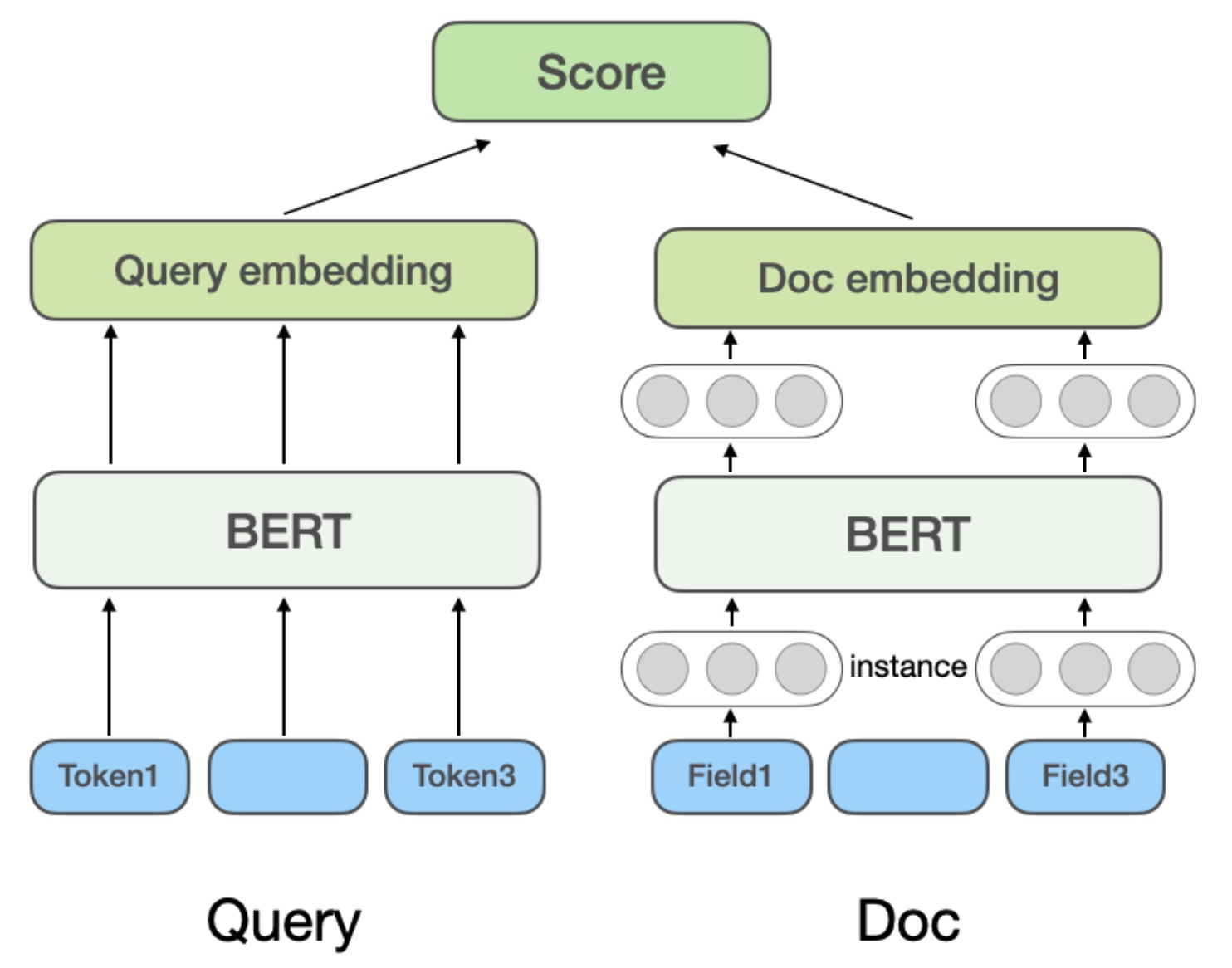
Representation-based method advantage: doc vectors can be offline computed and cached. Online serving only needs computing Query vector and simple similarity computation, good performance, low latency. Disadvantage: Query and Doc lack direct interaction during encoding, only relying on final vectors for similarity computation, might lose fine-grained matching signals, limited expressiveness.

• Interaction-based methods

This method doesn’t explicitly separate Query and Doc to learn semantic representation vectors, but lets them interact at bottom input stage. If dual-tower is retrieval paradigm, these models are ranking paradigm. ESIM was widely used before pretraining models. First encode Query and Doc to initial vectors, then use Attention for interaction weighting and concatenate with initial vectors, finally classify to get relevance score.

After introducing pretraining models like BERT, typically concatenate Query and Doc as BERT sentence relation task input, then input model to get final relevance score, as in Multi-Stage Document Ranking with BERT:

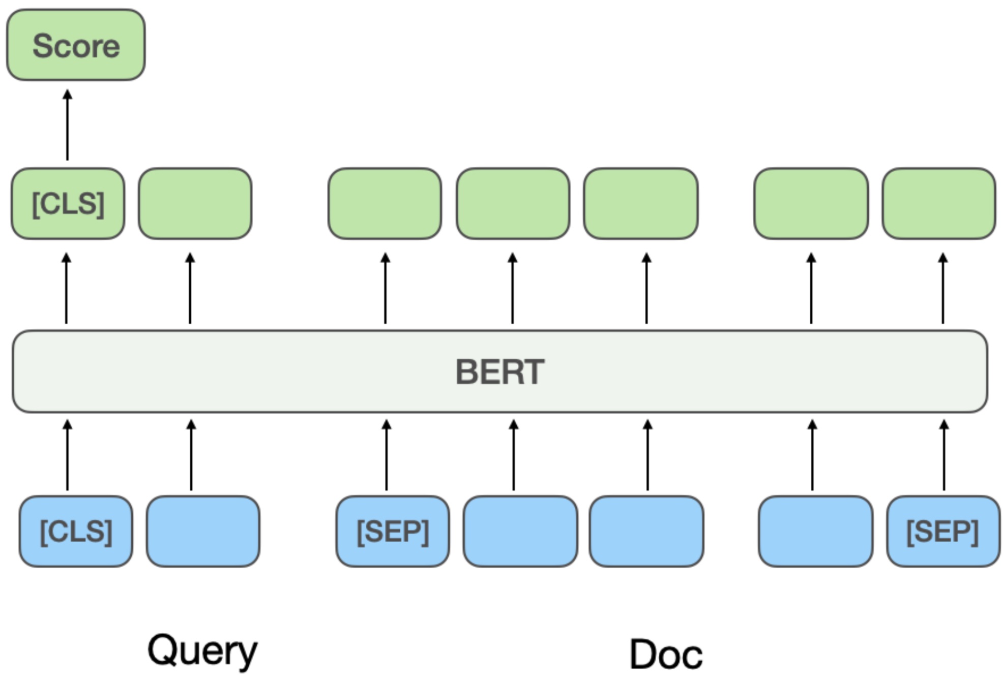
This method’s pros and cons are opposite to representation-based. Pros: High matching precision, capturing very fine-grained term interaction and deep semantic info. Cons: Huge computational cost. Online serving requires real-time Query-Doc concatenation and forward pass through large model, high latency, challenging performance.

Multi-Stage Training

Modeling needs solving basic problems including training sample acquisition, feature construction, model metrics. In relevance modeling, direct domain labeling data is costly, so multi-stage training is considered to improve model effectiveness while controlling cost.

• Training sample acquisition

Since relevance standards are platform-defined and frequently change, relevance training sample labels don’t have clear ground truth like CTR/CVR tasks, but rely on human annotation. And if standards change, labels might change, so training sample acquisition cost is high for specific domain relevance models.

Therefore, actual training often combines pretraining models + large easily-labeled relevant domain data for first stage, then human annotated data for second stage finetune. Taking Dianping article example (other domains are similar), first use user click and negative sampling data for Continual Domain-Adaptive Pre-training, then human annotated data for second stage Fine-Tune.

First stage training: This stage treats user click as “relevant” label, enabling low-cost large training sample acquisition. But directly using click samples for relevance judgment has significant noise, because user click is affected by many factors (most common is position - earlier positions more likely clicked, later not, but not due to relevance). So the approach introduces various features and rules to improve training sample accuracy. Specific rules:

For positive samples, filter candidates through statistics of click, click position, max clicked merchant distance from user, taking samples with impression CTR above threshold as positive. For negative samples, only take docs before clicked doc with CTR below threshold, while random negative sampling adds easy negatives, but also using human-designed rules for noise reduction: e.g., when Query category intent aligns with doc category system or highly matches doc name, exclude from negatives.

Second stage training: Second stage is common finetune training, fixing bottom layer parameters, using human-annotated more accurate labels to finetune top parameters. But different samples have different annotation value - easy pairs the model already judges well are less valuable than hard pairs the model can’t distinguish. So for annotation, Dianping doesn’t randomly send samples but produces high-value samples through hard example mining and contrastive sample augmentation for human annotation.

• Hard example mining: Including 1) samples user clicked but old model judged irrelevant; 2) edge sampling for highly uncertain samples like model prediction near threshold; 3) samples where model or human identified difficulty, using current model to predict training set, samples where prediction disagrees with label, and conflicting labels, sent for re-annotation
• Contrastive sample augmentation: Borrowing contrastive learning ideas, generating contrastive samples for highly matched samples and human annotating to ensure accuracy. Through contrastive sample differences, model can focus on truly useful info while improving synonym generalization. Example:

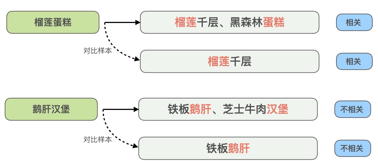
Here query “durian cake” is relevant to recommended “durian mille crepe, black forest cake”, but query “goose liver burger” is irrelevant to “iron plate goose liver, cheese beef burger”. To enhance model’s recognition of such highly matched but opposite result cases, the method constructs contrastive samples “durian cake” vs “durian mille crepe”, “goose liver burger” vs “iron plate goose liver”, removing info matching query text but unhelpful for model judgment, letting model learn key info determining relevance, while improving generalization for synonyms like “cake” and “mille crepe”.

• Features

Since relevance is relatively objective standard (given query and doc, posterior label is clear), not much affected by context info (like position, context). Or query and doc relevance won’t change due to different positions. Therefore, relevance model features are relatively simple - query features generally original query text, doc features generally doc multimodal info (title, image) and meta info (doc category, etc.).

With widespread LLM use, approaches using LLMs to construct additional query and doc features have emerged. For query, basic approach is constructing prompt based on query (e.g., based on query and various platform search results), then having LLM summarize and output more accurate detailed query summary, then using this as additional query feature input to relevance model.

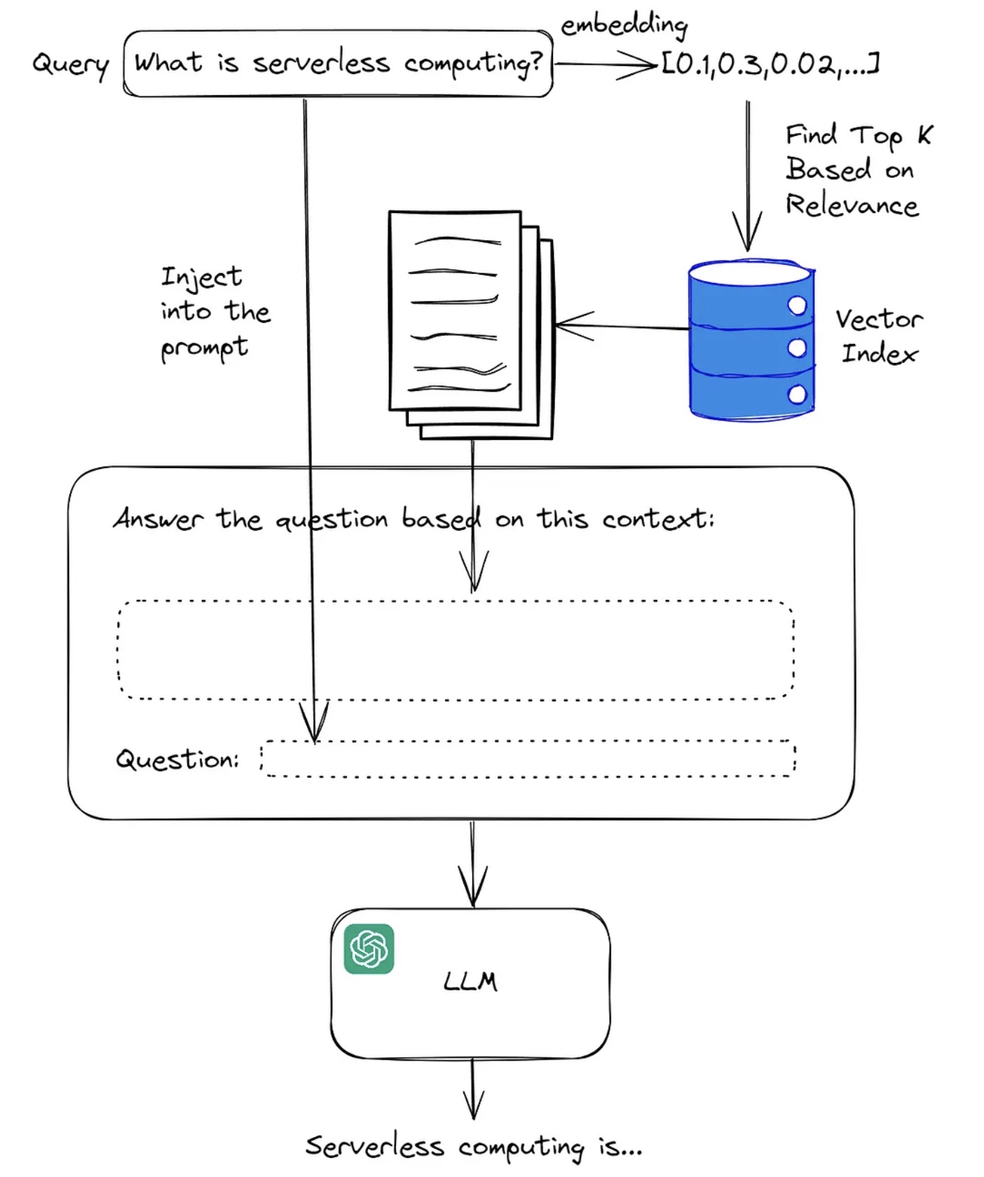
Industry practice generally uses RAG (Retrieval-Augmented Generation) for this step. RAG combines retrieval and generation. Basic workflow: when model receives query, first retrieves relevant documents or info fragments in large index, retrieval based on similarity measure to find most relevant info, then model uses retrieved documents as additional context input for generation, usually by LLM. frames basic workflow:

RAG technology through more detailed LLM input can alleviate LLM hallucination, also commonly applied in specific vertical search domains. For more RAG details, see Large Model RAG (Retrieval-Augmented Generation) with Advanced Methods.

Ranking Mechanism

With relevance estimates, next is how to apply them online. Systems generally ensure relevance through two means: relevance threshold and ranking formula adding relevance term.

• Relevance threshold: Fixed value, filtering low-relevance ad candidates
• Ranking formula adding relevance term: Dynamically changing value, controlling post-delivery relevance target achievement

Search relevance’s fundamental goal is ensuring agreed badcase rate constraint isn’t exceeded. If relevance score label is defined as whether badcase, estimate’s physical meaning is probability of badcase, becoming a very common binary task. Then when model estimates accurately, controlling posterior estimate mean to equal some target controls badcase rate around fixed value. E.g., if badcase target is 5%, with accurate relevance estimates, keeping relevance estimate mean at 0.95 achieves this.

What should the ranking mechanism be? Below provides a solution approach.

Optimal Ranking Formula

First, optimal ranking formula derivation, formalizing the problem. Taking ad scenario maximizing eCPM as example:

Assuming \(n\) requests, for request \(i\)’s shown ad, relevance estimate is \(predict\_rel\_score_i\), ad value is \(ecpm_i\), relevance mean target is target. The optimization problem formalizes as (decision variable \(x\) is ad selection strategy):

\[\begin{align} \max_x &\sum_{i=0}^{n-1} ecpm_i \\ s.t. \frac{1}{n} &\sum_{i=0}^{n-1} predict\_rel\_score_i=target \end{align}\]

Problem Modeling

Since each request often has multiple ads, the above problem can be further refined:

Assume request \(i\) has \(m_i\) candidate ads. For ad \(k\) in request \(i\), define:

• \(ecpm_{ik}\): Ad’s eCPM value
• \(s_{ik}\): Ad’s relevance estimate score (i.e., \(predict\_rel\_score\))
• \(x_{ik}\): Binary decision variable, \(x_{ik}=1\) means selecting ad \(k\) in request \(i\), otherwise \(x_{ik}=0\)

Then problem becomes:

\[\begin{align} \max &\sum_{i=0}^{n-1} \sum_{k} x_{ik} \cdot ecpm_i \\ s.t. &\sum_{i=0}^{n-1} \sum_{k} x_{ik} \cdot s_{ik} = (\sum_{i=0}^{n-1} \sum_{k} x_{ik}) \cdot target \\ & x_{ik} \in \{0,1\} \quad \forall i,k \end{align}\]

Problem Solving

1. Lagrangian Relaxation

Since constraint is equality and global, use Lagrangian multiplier to incorporate constraint into objective. Introduce Lagrangian multiplier \(\lambda\), construct Lagrangian function \(L\):

\[\begin{align} L(\mathbf{x}, \lambda) &= \sum_{i=0}^{n-1} \sum_{k} x_{ik} \cdot \text{ecpm}_{ik} + \lambda \left( \sum_{i=0}^{n-1} \sum_{k} x_{ik} \cdot s_{ik} - (\sum_{i=0}^{n-1} \sum_{k} x_{ik}) \cdot \text{target} \right) \\ &= \sum_{i=0}^{n-1} \sum_{k} x_{ik} \cdot (\text{ecpm}_{ik} + \lambda \cdot (s_{ik} - \text{target})) \end{align}\]

Here \(\lambda\) can be interpreted as “shadow price” of relevance constraint, meaning marginal impact on total eCPM per unit relevance score change. Maximizing \(L\) is equivalent to maximizing:

\[\begin{align} \max L(\mathbf{x}, \lambda) \iff \max \sum_{i=0}^{n-1} \sum_{k} x_{ik} \cdot (\text{ecpm}_{ik} + \lambda \cdot (s_{ik} - \text{target})) \end{align}\]

2. Problem Decomposition

For each request \(i\), maximizing \(\sum_{k} x_{ik} \cdot (\text{ecpm}_{ik} + \lambda \cdot (s_{ik} - \text{target}))\) is equivalent to selecting ad \(k\) maximizing \(\text{ecpm}_{ik} + \lambda \cdot (s_{ik} - \text{target})\):

\[\begin{align} k_i^* = \arg\max_{k} (\text{ecpm}_{ik} + \lambda \cdot (s_{ik} - \text{target})) \end{align}\]

Therefore, optimal decision is for each request \(i\), independently selecting ad \(k\) to maximize the linear combination, which is each request’s ranking formula:

\[\begin{align} score_{ik}=\text{ecpm}_{ik} + \lambda \cdot (s_{ik} - \text{target}) \end{align}\]

3. \(\lambda\) Solving

Mathematically, \(\lambda\) is Lagrangian multiplier obtained by solving constraint equation. In actual systems, \(\lambda\) can be adjusted through iterative methods (like binary search, gradient descent, or online learning). Binary search can be used (because \(s_i(\lambda)\) is monotonically increasing in \(\lambda\)):

1. Initialize \(\lambda_{low}\) and \(\lambda_{high}\)
2. For each \(\lambda\), compute all requests’ selections (maximizing \(\text{ecpm}_{ik} + \lambda \cdot s_{ik}\)) and compute mean \(s_i\)
3. If mean \(s_i > \text{target}\), decrease \(\lambda\) (reduce relevance weight); otherwise increase
4. Repeat until mean \(s_i\) converges to target

The above method requires obtaining all traffic and candidates, equivalent to replaying past period’s traffic to get historical optimal exchange ratio \(\lambda\). But like optimal bidding, this is hard to directly apply because two prerequisites: (1) get all current day’s traffic data (2) changing actual winning ads won’t affect bidding environment. These are often hard to satisfy.

More common practice is collecting relevance estimate mean from past period, then using PID for real-time control adjusting \(\lambda\), pacing target being relevance mean equals target. This is similar to bidding control, also leading to gap between actual and theoretical optimal exchange ratio, requiring various approaches to approach theoretical optimal.

Approaching Theoretical Optimal

Analyzing further, actual PID control vs replay optimization differs in whether the control process perceives traffic value i.e., eCPM.

Because optimization solving has maximizing eCPM objective in constraint solving, searching for \(\lambda\) just satisfying target. But actual controller control only perceives current relevance mean achievement. When relevance isn’t achieved, \(\lambda\) gets very large, making eCPM term’s role in ranking very small, leading to non-optimal eCPM.

For example, in two consecutive time slices, first time relevance not achieved but has high eCPM candidates. Only considering relevance, \(\lambda\) gets very large, preventing high eCPM candidates from showing (relevance term dominates). Next time slice relevance improves (because first slice showed high relevance ads), but candidates have no high eCPM. Now lower relevance weight, but shown ads’ eCPM isn’t optimal either. But if reversed - first lower \(\lambda\), second raise \(\lambda\), can achieve balanced relevance with maximized eCPM. This requires control perceiving traffic value.

Perceiving traffic value in \(\lambda\) control, most intuitive is using collected traffic and ad candidates from past period \(t\), then directly solving optimization via binary search above for optimal exchange ratio \(\lambda^*\), used for next time slice. But this has strong assumption that past period \(t\)’s traffic and candidate distribution is similar to next time slice (or small difference) to be effective.

Besides above method, another more intuitive approach is dynamically adjusting exchange ratio based on traffic value during control. If partitioning traffic by value and relevance, we get four quadrants:

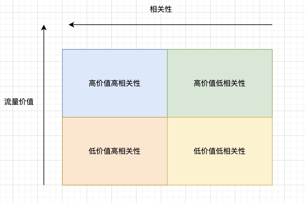
For these four traffic types, intuitively we can give prior exchange principles:

1. High value high relevance: Lower exchange ratio, maximize high eCPM ad delivery
2. Low value high relevance: Raise exchange ratio, maximize high relevance ad delivery to fill high relevance
3. High value low relevance: Lower exchange ratio, but higher than (1), prevent relevance not achieved
4. Low value low relevance: Raise exchange ratio, higher than (2), minimize ad delivery

This contradicts theoretical optimal derivation conclusion “global optimal exchange ratio is fixed \(\lambda\)”. Because we’re giving different exchange ratios for high vs low value traffic, not globally unified. But actually theoretical optimal assumption (see all traffic) can’t be satisfied, and we’re approximating theoretical optimal, so don’t need to follow fixed \(\lambda\) conclusion.

Additionally, this method’s effectiveness has two important assumptions: 1) Relevance lost from high value traffic can be recovered from low value traffic; 2) Unit relevance has higher exchange efficiency in high value than low value traffic. Point 1 is straightforward - if can’t recover, relevance can’t be achieved. Point 2 means eCPM and relevance score distributions differ between high and low value, or intuitively: getting unit relevance in high value traffic costs larger \(\Delta eCPM\) than low value traffic. This depends on actual inventory distribution (eCPM and relevance score distribution). From actual systems, this assumption likely holds.

Also, actual control needs to ensure overall target is achievable after these exchange ratio adjustments. From this perspective, approach 2 better achieves this than approach 1, because can perturb based on unified control coefficient. Approach 2’s solution is similar to “protect shallow optimize deep” perturbation strategy in bidding, perturbing \(\lambda\) based on traffic value while ensuring overall target achievement. But unlike bidding done at plan level, relevance is overall level, can’t be done at plan level. First, target is overall constraint, can’t decompose well to individual plans. Second, doing at plan level isn’t optimal because each plan needs its own target, adding more constraints and smaller solution space. For similar approaches in bidding, see Bid Optimization by Multivariable Control in Display Advertising.

Summary

This article discusses relevance modeling technology evolution and optimal control strategies in ranking mechanisms, attempting to provide systematic solution approaches for this classic problem. Starting from search vs recommendation scenario differences, search scenario’s strong intent characteristic determines relevance’s special nature: unlike recommendation’s “purposeless browsing”, user search has clear expectations, requiring results precisely match query intent. From technical perspective, this divides into relevance modeling and ranking mechanism.

In relevance modeling, basic evolution goes from text matching to deep semantic matching. Current mainstream methods divide into representation-based and interaction-based paradigms, each trading off precision vs performance. After introducing pretraining models and RAG technology, model understanding depth and generalization for semantics significantly improve. Two points deserve attention in relevance modeling: First, LLM-based semantic understanding and generation: LLMs show strong capability in semantic understanding, intent inference, and content generation. Future may deeply apply LLMs for deep query intent parsing, expansion, and normalization, even directly generating or enhancing relevant content summaries, further improving relevance judgment accuracy and interpretability. Second, personalized relevance understanding: Search intent has group commonality but also individual differences. Although current relevance isn’t context-dependent, future relevance models may better integrate personalized context (like history, real-time preferences), providing results more aligned with individual needs while ensuring basic relevance.

In ranking mechanism, the optimization problem formalization derives ranking formula with relevance constraint \(score =\text{ecpm} + \lambda \cdot \text{rel\_score}\). The Lagrangian multiplier \(\lambda\) can be considered “shadow price” of relevance constraint, achieving balance between relevance target and eCPM maximization through \(\lambda\) control.

Current \(\lambda\) control is mostly based on overall mean, hard to perceive traffic value differences. Ideal state achieves fine-grained control by traffic value tier - for high value high relevance traffic lower \(\lambda\) to improve eCPM, for low value high relevance traffic raise \(\lambda\) to ensure relevant experience. Meanwhile need to consider not breaking overall target while achieving dynamic control.

Search ad relevance, ultimately, is the art and science of finding best balance among user intent, advertiser needs, and platform value. It requires both deep technical modeling and algorithm optimization, and deep insight into user search psychology and advertiser business objectives. Future search ad systems may be more intelligent and adaptive, dynamically sensing different scenarios and users’ differentiated relevance expectations, precisely controlling business-experience balance point.