Generative Recommendation (GR): What It Actually Replaces, and What It Doesn't
“Generative Recommendation” has been one of the most frequently used terms in recommender systems over the past year, but it actually refers to completely different things depending on who is speaking. A paper about plugging LLMs into recommendation calls it “generative recommendation”; a work using RQ-VAE to build semantic IDs also calls it “generative recommendation”; an industrial system that merges recall-ranking-reranking into a single encoder-decoder also calls it “generative recommendation”.
But these three things have essentially no intersection in their engineering meaning.
When they are mixed together, two common but imprecise judgments appear:
- One is “GR is just hype, industry can’t use it”
- The other is “the cascade paradigm is about to be completely overturned”
Both judgments assume “GR” is one thing. But if you unpack it slightly, you find: semantic ID has been deployed in several companies, HSTU has been deployed at Meta, OneRec has been deployed at Kuaishou (at least according to the papers), while most LLM-as-Recommender type works still have very little industrial deployment evidence. Clearly this is not a 0/1 question of “is GR hype” that can be answered.
So what this article really wants to discuss is not “is GR the future”, but a more specific set of questions: After cascade (recall - coarse ranking - fine ranking - reranking) has supported industrial recommender systems for over a decade, which assumption is GR actually challenging? What does it replace, and what does it not replace? What has been validated industrially, and what remains at the paper level?
To avoid the chapter-level details drowning out the main thread, let me state the full article’s thesis up front: GR is not a wholesale replacement of cascade, but rather it opens a “use generative modeling to re-frame” door for each layer of cascade. But the industrial difficulty behind each door varies enormously; it must be examined layer by layer, not as a single thing.
Three Implicit Assumptions of the Cascade Paradigm
To understand what GR is challenging, we first need to unpack the implicit assumptions of the cascade paradigm. The reason the cascade paradigm works well is that at least three long-standing implicit assumptions hold behind it.
Assumption A: Items are Discrete Atoms
In cascade systems, each item is represented by a hash ID + embedding, and semantic relationships between items are slowly learned entirely through collaborative signals. This has worked for over a decade, but the preconditions are:
- Behavioral signals are dense enough that each item can accumulate sufficient co-occurrence
- Item vocabulary growth is controllable, the embedding table can handle it
- The long tail is unimportant, new items are a low fraction, or cold-start can be backed by side features
These three preconditions are actually starting to waver on large-scale, UGC-driven modern content platforms. The number of new items added daily, the long-tail fraction, cross-domain transfer needs—all make the hash ID system increasingly strained.
Assumption B: Each Step Can Be Scored Independently
This is exactly what the previous article 《Personalized Ranking Formula: From Personalized Fine-Ranking to Personalized Mixed-Ranking to Global Re-Ranking》 discussed: the first layer does pointwise \(s(u,i,x)\), the second layer does mixed ranking, the third layer does listwise / Slate. This assumption actually contains two layers:
- B1: Each item can be scored independently (pointwise) — given \((u, i)\), the model gives a single score, not depending on other items in the list
- B2: Multi-step cascade approximates global optimum — recall, ranking, reranking are layered, assuming “sum of local optima ≈ global optimum”
The reason this layering works is that cascade assumes local optimum approximates global optimum.
But intra-list item-item interactions cannot be ignored — fatigue, complementarity, substitution, position dependence — this assumption breaks down. So listwise re-ranking, Generator-Evaluator, Slate optimization are forced to graduate from “post-processing tools” to “first-class citizens”.
Assumption C: Recommender Systems Do Not Exhibit a Significant Scaling Law
This is a fact that has long been unwilling to admit but always accepted: DLRM-style models have long been saturated in scaling along the parameter dimension.
Meta’s 2022 Understanding Scaling Laws for Recommendation Models (Ardalani et al., arXiv:2208.08489) systematically quantified this for the first time — DLRM model quality in the data and compute dimensions still follows a power law + constant form, but parameter-dimension scaling has already gone “out of steam”, and continued parameter increase brings rapidly diminishing marginal returns. The HSTU paper again demonstrated the same phenomenon in its own baseline experiments: the quality-compute curve of traditional DLRM quickly enters a plateau, while HSTU’s curve continues to follow a power law over three orders of magnitude in compute.
This is also the fundamental reason recommender models have long remained at the hundred-million-parameter scale — not that bigger isn’t wanted, but that bigger brings no gain. The subtle point: it’s not that “recommendation data isn’t enough”, but that “the expressiveness of traditional DLRM architecture on large-scale behavior sequences is limited by its own design”.
What GR really challenges happens to be exactly these three assumptions:
| Assumption | Cascade Presupposition | How GR Challenges |
|---|---|---|
| A. Item is a discrete atom | hash ID + emb, no structure | semantic ID (RQ-VAE), hierarchical tokens |
| B. Each step can be scored independently | recall→rank→rerank cascade | HSTU challenges B1 (sequence modeling replaces pointwise); OneRec challenges B2 (end-to-end generation of whole list) |
| C. No scaling law | DLRM bigger may not be better | HSTU validates power-law over three orders of compute |
These three assumptions are not challenged simultaneously, and the corresponding GR works are not the same kind. We will see that the industrial evidence for semantic ID is fairly substantial; HSTU challenges B1 and C with real deployment cases at Meta; while the public industrial evidence for “end-to-end generation of the whole list” (challenging B2) mainly comes from the Kuaishou OneRec technical lineage, with cross-company independent validation still limited. These three things are not the same.
GR Reframes Recommendation as “Sequence Generation”
The core paradigm of GR can be roughly stated in one sentence: reframe recommendation from “scoring and sorting candidate items” to “generative prediction on user behavior sequences”.
But more rigorously, GR has at least two layers — broad and narrow:
- Broad GR: reframes recommendation from independent \((u,i)\) discriminative scoring to next-action / sequential transduction on user behavior sequences. HSTU belongs to this layer; it does not necessarily generate item tokens.
- Narrow GR: further lets the model autoregressively generate item tokens / semantic IDs, then map back to real items. TIGER and OneRec belong to this layer.
Written in the narrow item-token generation form, it can be expressed as:
\[ p(i_t \mid i_{<t}, u) = f_\theta\big(\text{tokenize}(i_{<t}),\, u\big) \]
Symbol definitions:
- \(i_t\): the \(t\)-th item to be generated (i.e., “the next content recommended”)
- \(i_{<t}\): the user’s historical interaction sequence (usually an item list sorted by time)
- \(\text{tokenize}(\cdot)\): item tokenizer, mapping a single item to several discrete tokens
- \(u\): user-side information (can be user ID, profile, context, etc.)
- \(f_\theta\): autoregressive generative model or sequence prediction model (TIGER / OneRec directly generate item tokens; HSTU is closer to broad next-action sequence prediction)
In plain terms, the traditional cascade view is:
“Give me a pile of candidate items, I’ll score each one and output a sorted list.”
The narrow GR view is:
“Give me the user’s past behavior sequence, I directly generate the next item (or the next segment of items).”
Broad GR and traditional cascade already differ in mathematical form; narrow GR differs even more in engineering implementation. The following comparison table is the backbone of the article:
| Dimension | Discriminative Cascade | Generative Recommendation GR (typical form) |
|---|---|---|
| Item representation | hash ID + dense emb | semantic ID (narrow GR) / action token (broad GR) |
| Single decision object | score of single \((u, i)\) | next action / token |
| List generation | recall → ranking → reranking cascade | autoregressive decode (can generate the whole segment at once) |
| Training objective | multi-objective weighted loss | next-token cross-entropy (+ subsequent reward alignment) |
| Scaling Law | empirically weak | HSTU validated at GPT-3-level compute |
| Inference form | matrix multiplication + ANN retrieval | autoregressive decode + beam search |
| Cold start | relies on side features | semantic ID carries semantic hierarchy |
A boundary clarification is needed here to avoid being misled by the literal meaning:
- GR ≠ “plugging LLMs into recommendation”. LLM-as-Recommender is only one form of GR; HSTU, trained from scratch on recommendation data, does not even depend on a general LLM
- GR ≠ “end-to-end overthrow of cascade”. Even an end-to-end GR like OneRec still retains business-level mixed ranking and constraint fallback mechanisms
- GR ≠ “must use semantic ID”. Most of HSTU’s official implementation is still hash-based; it challenges assumptions B and C, not A
In other words, GR is a paradigm collection, not a single architecture. The following three technical pillars correspond to three independent but mutually cooperating technical lines within this paradigm.
Three Key Questions
For GR to land industrially, it essentially needs to solve three things, which exactly correspond to the three core components of the GR paradigm:
- How to represent items as tokens that the model can generate? (Item Tokenization) — corresponds to the “item representation” component
- What architecture to use for this sequence generation? (Generative Architecture) — corresponds to the “sequence modeling” component
- How does the decoded token sequence correspond back to real items? (Decoding & Inference) — corresponds to the “token fall-back” component
Each of these has its own mature methods, representative works, and deployment difficulty, must be examined separately, not mixed together to judge whether GR is mature. This is also why earlier we said “semantic ID is already industrially deployed, HSTU is already deployed, but end-to-end GR independent validation is still limited” — the maturity of the three components is completely different.
Item Tokenization: Semantic ID and RQ-VAE
Core question: why can’t hash ID support GR?
The fundamental problem with hash IDs is that adjacent IDs have no semantic relationship. In discriminative cascade this is fine — the embedding is looked up anyway, the ID itself is just a query index, whether adjacent IDs look alike or not doesn’t matter.
But in the GR paradigm, what the model does is “generate IDs”. This requires the ID space itself to have structure: similar items should have similar IDs, so the model can infer from “has seen A” that “probably also likes B similar to A”. Hash IDs inherently lack this property, so they must be replaced.
RQ-VAE Principle
Residual-Quantized VAE (RQ-VAE) is currently the most mainstream item tokenizer in GR. The principle can be split into two steps.
Step 1: train a content encoder \(E\)
It takes the item’s content information (text description, image, behavioral statistics, category, etc.) and outputs a dense embedding:
\[ z = E(i) \]
Step 2: residual-quantize \(z\) into \(L\) codebook indices
\[ \begin{aligned} r_0 &= z \\ c_l &= \arg\min_k \big\| r_{l-1} - e_k^{(l)} \big\| \quad l = 1, \dots, L \\ r_l &= r_{l-1} - e_{c_l}^{(l)} \end{aligned} \]
Symbol definitions:
- \(r_l\): the residual vector at layer \(l\)
- \(e_k^{(l)}\): the \(k\)-th vector in the \(l\)-th codebook (each codebook is a learnable vector dictionary)
- \(c_l\): the codebook index matched at layer \(l\)
- \(L\): number of codebook layers, typically 3-4 in industrial implementations
Each item is finally represented as a token tuple \((c_1, c_2, \dots, c_L)\), called this item’s semantic ID.
The whole quantization process is a greedy process of “approximating \(z\) layer by layer with codebooks”. Each step does the same thing: “how much of \(z\) is not yet encoded? Find the closest code in the current codebook to fill it in”. Unpacking it:
- Initialization: \(r_0 = z\), meaning “nothing encoded yet, the entire \(z\) is to be encoded”.
- Layer 1: pick a code \(e_{c_1}^{(1)}\) from codebook 1 closest to \(r_0\), \(c_1 = \arg\min_k \|z - e_k^{(1)}\|\). Then compute “the unencoded part”: \(r_1 = z - e_{c_1}^{(1)}\).
- Layer 2: layer 1 has “used up” the \(e_{c_1}^{(1)}\) block, the remaining \(r_1\) still needs to be approximated. So layer 2 picks the code closest to \(r_1\) from codebook 2: \(c_2 = \arg\min_k \|r_1 - e_k^{(2)}\|\), new residual \(r_2 = r_1 - e_{c_2}^{(2)}\).
- Layer \(L\): and so on, each layer “takes over” the residual left by the previous layer.
After walking through \(L\) layers, summing all hit codes approximately restores \(z\):
\[ z \approx \sum_{l=1}^L e_{c_l}^{(l)} \]
That is, semantic ID \((c_1, \dots, c_L)\) is essentially a set of discrete indices, telling you “how to reassemble \(z\) using vectors from \(L\) codebooks”. The closer the reconstruction is to \(z\), the more semantic information the semantic ID preserves.
Here is a simple K=3, L=3 example:
- \(z = (1.0,\ 0.8)\)
- codebook 1 = \(\{(1.0,\ 1.0),\ (-1.0,\ 0.0),\ (0.0,\ -1.0)\}\)
- codebook 2 = \(\{(0.1,\ -0.1),\ (-0.1,\ 0.1),\ (0.2,\ 0.0)\}\)
- codebook 3 = \(\{(0.05,\ -0.05),\ (-0.05,\ 0.0),\ (0.0,\ 0.05)\}\)
The semantic ID construction is as follows:
- Layer 1: \(r_0 = (1.0,\ 0.8)\). Distances from the three candidate codes to \(r_0\) are approximately \(0.20,\ 2.15,\ 2.06\); the closest is the first, so \(c_1 = 1\). Residual \(r_1 = (1.0,\ 0.8) - (1.0,\ 1.0) = (0.0,\ -0.2)\).
- Layer 2: \(r_1 = (0.0,\ -0.2)\). Distances are approximately \(0.14,\ 0.32,\ 0.28\); the closest is the first, so \(c_2 = 1\). Residual \(r_2 = (0.0,\ -0.2) - (0.1,\ -0.1) = (-0.1,\ -0.1)\).
- Layer 3: \(r_2 = (-0.1,\ -0.1)\). Distances are approximately \(0.16,\ 0.11,\ 0.18\); the closest is the second, so \(c_3 = 2\).
Final semantic ID is \((1,\ 1,\ 2)\). Reconstruction:
\[ \hat{z} = (1.0,\ 1.0) + (0.1,\ -0.1) + (-0.05,\ 0.0) = (1.05,\ 0.9) \]
The reconstruction error from the true \(z = (1.0,\ 0.8)\) is \(\|z - \hat{z}\| \approx 0.11\) — the more layers and the larger the codebook, the closer the reconstruction to \(z\), and the finer the information encoded in the semantic ID.
Several key points about this process:
- Greedy quantization: each step only looks at “which code is closest in this layer”, without jointly considering subsequent layer choices. In theory joint optimization gives more accurate reconstruction, but the combinatorial space is \(K^L\), infeasible; the greedy scheme is not globally optimal but training and inference are both \(O(L \cdot K)\), which is the only thing affordable in practice.
- Quantization is lossy: each layer leaves a residual \(\|r_l - e_{c_l}^{(l)}\|\). The larger \(L\) and \(K\), the more accurate the reconstruction, but the longer the token sequence and the slower the decoding — this is the fundamental trade-off in RQ-VAE engineering parameters.
In plain terms: it’s like classifying a book first by coarse category (“novel”), then within the coarse category by medium category (“mystery novel”), then within the medium category by fine category (“locked-room mystery”). Each layer uses a small vocabulary to depict a specific granularity of semantics. Semantically adjacent items will overlap on prefix tokens, and the model naturally learns the structure that “similar items have similar IDs”.
Why “residual + multi-layer” rather than one large codebook
There is a natural question here: if you want \(K^L\) different IDs, why not just use a single codebook of size \(K^L\) and quantize once?
The answer lies in structure and generalization. A single-layer codebook of size \(K^L\) needs to learn \(K^L\) independent vectors, each item hits only one of them, and there is no relationship between adjacent IDs — this essentially degenerates back to hash ID.
RQ-VAE is different: each layer only learns \(K\) vectors, with total parameter count \(L \cdot K\), but through combination yields \(K^L\) semantic IDs. More importantly, layer \(l\) only encodes information not captured by the first \(l-1\) layers — this is the full meaning of “residual”. And precisely because of this progressive structure, prefix tokens naturally carry coarse-grained semantics.
How to train
RQ-VAE is trained end-to-end with encoder + \(L\) codebooks + decoder. Here the decoder reconstructs the item’s continuous representation \(z\) (or the item feature representation corresponding to \(z\)). The loss consists of three parts:
\[ \mathcal{L}_{\text{RQ-VAE}} = \underbrace{\|z - \hat{z}\|^2}_{\text{reconstruction}} + \underbrace{\sum_l \|\text{sg}(r_{l-1}) - e_{c_l}^{(l)}\|^2}_{\text{codebook learning}} + \underbrace{\beta \sum_l \|r_{l-1} - \text{sg}(e_{c_l}^{(l)})\|^2}_{\text{commitment}} \]
- \(\hat{z}\): the item representation reconstructed by the decoder using the quantized \(\sum_l e_{c_l}^{(l)}\)
- \(\text{sg}(\cdot)\): stop-gradient, blocking gradient backpropagation
- \(\beta\): commitment weight, VQ-VAE default 0.25
Plain explanation:
- Reconstruction loss makes the whole codebook combination able to restore the item representation
- Codebook learning loss makes each codebook vector slowly approach the mean of residuals that actually hit it
- Commitment loss conversely constrains the encoder output not to drift too far from the codebook
The quantization operation \(\arg\min\) is discrete and non-differentiable, solved in engineering by the straight-through estimator (STE): forward pass uses the quantized value, backward pass lets gradients directly bypass the quantizer to reach the encoder. This is a standard trick inherited from VQ-VAE.
Where do the codebook vectors come from
The \(L\) codebooks are not pre-defined dictionaries, but trainable parameters learned end-to-end together with the encoder / decoder. The learning process of each codebook is intuitively equivalent to K-means clustering in residual space — the \(K\) codes slowly evolve into “the cluster centers of \(K\) common residuals”. Concretely, the \(\sum_l \|\text{sg}(r_l) - e_{c_l}^{(l)}\|^2\) term in the loss above can directly do gradient updates, or EMA can maintain the code as “the mean of all residuals that hit it over a recent period” (the VQ-VAE paper recommends the latter as more stable).
After training, the codebook is generally frozen, and all items are quantized using this fixed codebook. But industrially, note that as item distribution drifts and new categories appear, the quantization quality of the original codebook gradually degrades — periodic retraining of RQ-VAE at weekly / monthly scale is needed, and after retraining, the semantic IDs of all items must be globally recomputed. This is an engineering cost that cannot be ignored.
Common values for engineering parameters
In industrial deployment there are several relatively converged empirical values:
| Parameter | Common value | Note |
|---|---|---|
| Codebook size \(K\) | 256 (or 512) | Too small = insufficient expressiveness; too large = prone to collapse |
| Number of layers \(L\) | 3-4 | TIGER uses 4 layers |
| Effective vocabulary \(K^L\) | \(\sim 10^9\) order | Enough to cover ten-billion-scale item pools |
| Commitment weight \(\beta\) | 0.25 | VQ-VAE default |
| Codebook vector dimension | 32-128 | Determined by content encoder output dimension |
That is, a typical configuration (\(K=256, L=4\)) yields about 4.3 billion different semantic IDs, far exceeding the item scale of typical recommender systems.
The biggest pitfall in industrial deployment: codebook collapse
This is the most common problem in actual RQ-VAE deployment and the least discussed in papers.
Symptom: after several training rounds, a few codebook vectors get repeatedly hit, while others are almost never used. For example, of 256 codes, only 30 are actually active. This is equivalent to cutting the effective vocabulary from \(K^L\) to \(30^L\), with expressiveness dropping sharply, and the hierarchical structure of semantic IDs also collapses.
Root cause: \(\arg\min\) is winner-take-all. Once a code is hit more in the early stage, its update direction shifts toward the average vector of items that hit it, and next round it’s more likely to be hit again, forming positive feedback.
Common mitigation methods:
- Codebook reset: periodically replace long-unused codes with “the hardest-to-explain residual vectors” (reservoir sampling)
- EMA update: use exponential moving average to smooth codebook learning, avoiding being dominated by a few batches
- K-means initialization: initialize the codebook with K-means centers of training-set residuals, avoiding cold-start bias
- Entropy regularization: add a term to the loss encouraging the entropy of the code hit distribution
These methods are mentioned in the original RQ-VAE paper and follow-up works, but the actual ratio and trigger conditions highly depend on the specific business’s item distribution, often requiring repeated tuning online.
Representative Work: TIGER
TIGER (Rajput et al., NeurIPS 2023, arXiv:2305.05065) is the earliest and most representative work in this paradigm. It does three things:
- Use RQ-VAE to generate a semantic ID for each item
- Use a T5-style autoregressive transformer to learn “given a historical behavior sequence, generate the next item’s semantic ID”
- At inference, use beam search to generate candidate semantic IDs, then map back to real items
TIGER’s real paradigm-level contribution, not some specific number, is that it proved one thing:
Transformer memory itself can serve as a semantic index — no separate ANN index is needed; the model parameters themselves take on the recall task.
This is almost unimaginable under the traditional cascade view: the recall side has been the “embedding + ANN” paradigm for over a decade, and TIGER first replaced it wholesale with “generative decoding”.
TIGER’s engineering details are as follows:
- Content encoder: sentence-T5, encoding item text descriptions into 768-dim vectors
- Then projected to 32-dim space for RQ
- \(K = 256\), \(L = 4\)
- To avoid different items being quantized to exactly the same semantic ID (hash collision), TIGER adds an additional disambiguating token to each ID tuple (effectively becoming 5 tokens)
The last detail is actually quite important: even with an effective vocabulary of \(K^L \approx 4 \times 10^9\), different items will still be quantized to the same ID, requiring extra tokens to distinguish. This is also why in the paper many semantic IDs are actually 4-5 tokens rather than a clean 4 — such “patches” are the norm in industrial implementation.
Limitations
Semantic ID is not a panacea; several of its engineering boundaries need to be seen clearly:
- Trade-off between vocabulary size and expressiveness: the number of codebook layers \(L\) and per-layer size \(K\) determine the effective vocabulary \(K^L\). Too small \(L\) = insufficient expressiveness; too large \(L\) = token sequence too long, decode slow
- Strong dependence on content encoder quality: items with weak behavioral signals and weak content signals (e.g., pure ID-type short content) still cold-start
- Codebook drift: after the model goes online, how to assign semantic IDs to new items? Whether to periodically retrain the codebook? These are pits not discussed in papers but inevitably encountered industrially
Finally, RQ-VAE was not invented by GR; it has been mature in images (VQ-VAE) and speech for years. The problem it solves — “discrete items have no structure” — is the prerequisite for the TIGER / OneRec “generate item token” line to hold. The scaling law of the HSTU line is relatively orthogonal to semantic ID; but for routes that need to autoregressively generate items, without semantic ID, subsequent constrained decoding, transformer-as-index, and end-to-end slate generation are all hard to establish. In addition, even if a team doesn’t plan to switch to full GR, first injecting semantic ID as a side feature into the existing cascade can already yield cold-start and long-tail gains.
Three Routes of Generative Architecture
The “architecture” pillar of GR is currently clearly divided into three routes. They are all formally called “generative”, but they solve fundamentally different problems, and their deployability differs enormously. Below they are introduced in descending order of industrial deployability.
Route 1: Training a Generative Foundation Model on Recommendation Data
The representative work is Meta HSTU (arXiv:2402.17152, “Actions Speak Louder than Words”). The main thing it does: reframe the DLRM-era “sparse features + multi-tower scoring” into “sequence modeling on user behavior sequences”, then use a transformer variant customized for recommendation scenarios to scale it up.
First clarify an easily misunderstood point: “generative” in HSTU does not mean it generates natural language like an LLM, nor does it mean it must generate RQ-VAE semantic IDs. What it does is a deeper reframing: treats user historical behavior as a string of action tokens, and the model predicts future actions based on past action sequences. Here the action can include item ID, action type, timestamp, scenario, device, context features, and other high-cardinality sparse information.
That is, the input of a traditional DLRM/ranker is more like a “feature table for the current request”:
\[ s(u, i, x) = f_\theta(\text{user features}, \text{item features}, \text{context}) \]
HSTU’s input is more like a behavior stream unfolded over time:
\[ x_t = \mathrm{Embed}(i_t, a_t, c_t, \Delta t_t, \dots) \]
Symbol definitions:
- \(i_t\): the item of the \(t\)-th interaction
- \(a_t\): interaction action, e.g., impression, click, completion, like, purchase
- \(c_t\): the context at the time, e.g., entry, device, region, scenario
- \(\Delta t_t\): time interval or time position feature
- \(x_t\): the \(t\)-th action representation after fusing these sparse features
The training objective also changes. A traditional ranker more commonly “scores the current candidate item”; HSTU is:
\[ p(x_{t+1} \mid x_{\le t}) = f_\theta(x_1, x_2, \dots, x_t) \]
In plain terms, it’s not just asking “will this user click this item now”, but asking “given this user’s path so far, what action is most likely to happen next”. This is where HSTU is closer to generative modeling than a traditional pointwise ranker.
Under this framework, HSTU makes three key changes relative to the standard Transformer. The key to understanding these changes: each change corresponds to a “standard Transformer mismatch in recommendation scenarios” — HSTU didn’t change things for the sake of changing them, but because default assumptions reasonable in NLP become obstacles in recommendation scenarios. The three changes below are examined in descending order of importance.
Change 1: Training Objective from “Per-Sample Scoring” to “Behavior Sequence Transduction”
The training paradigm of a traditional ranker
The traditional ranker’s training paradigm is “per-sample scoring”: each \((u, i, \text{label})\) sample independently contributes a binary classification loss (click / no-click). The underlying assumption is “each sample is independent, the objective can be decomposed into per-sample accumulation”.
HSTU changes to “sequence transduction”
“Sequential Transducers” in the HSTU paper title hints at a more fundamental shift: the training objective changes from “per-sample classification” to “sequence transduction”. Transducer means: given a historical behavior sequence, output the distribution over future behaviors or target actions — not just serving a single binary CTR objective, but unifying multiple recommendation tasks (click, completion, like, conversion, …) into a prediction problem on the sequence.
Seeing the difference through a concrete example
This difference is most easily masked by the surface similarity of “both use CE loss”, so let’s use a concrete example. Suppose the online log has the following user behavior:
User U in a certain session did 4 actions in sequence: 1. Watched basketball video A, completed 2. Watched basketball video B, liked 3. Watched food video C, skipped 4. Watched basketball video D, completed
Pointwise ranker’s approach — splits this session into 4 independent samples:
| Sample | User | Item | Label |
|---|---|---|---|
| 1 | U | Basketball A | 1 (completed) |
| 2 | U | Basketball B | 1 (liked) |
| 3 | U | Food C | 0 (skipped) |
| 4 | U | Basketball D | 1 (completed) |
These 4 samples can be shuffled in a batch — they are completely equivalent in status to a sample like “user V skipped game E”. Each sample independently computes a binary CE, and they sum to the batch loss:
\[ \mathcal{L}_{\text{pointwise}} = -\big[\log \sigma(s(U, A)) + \log \sigma(s(U, B)) + \log(1 - \sigma(s(U, C))) + \log \sigma(s(U, D))\big] \]
The history sequence (if used) only enters as a feature into \(s(U, \cdot)\) and does not participate in loss construction.
HSTU’s approach — treats the entire session as one training sample, no splitting. Each position contributes a “predict next step” loss term:
| Position \(t\) | Input | Predict target | Loss term |
|---|---|---|---|
| 1 | \(x_1\) (watch basketball A complete) | \(x_2\) (watch basketball B like) | \(-\log p(x_2 \mid x_1)\) |
| 2 | \(x_1, x_2\) | \(x_3\) (watch food C skip) | \(-\log p(x_3 \mid x_1, x_2)\) |
| 3 | \(x_1, x_2, x_3\) | \(x_4\) (watch basketball D complete) | \(-\log p(x_4 \mid x_1, x_2, x_3)\) |
\[ \mathcal{L}_{\text{HSTU}} = -\big[\log p(x_2 \mid x_1) + \log p(x_3 \mid x_1, x_2) + \log p(x_4 \mid x_1, x_2, x_3)\big] \]
A sequence of length \(T\) contributes \(T-1\) loss terms, each position being a multi-class classification task of “given the first \(t\) steps of history, predict the \(t+1\)-th step”.
Three differences between the two methods:
| Dimension | Pointwise ranker | HSTU |
|---|---|---|
| Can samples be shuffled | Yes, session split into independent samples | No, order is part of the loss |
| Loss form | binary CE accumulated per-sample | multi-class CE at each position |
| How many loss terms per session | \(T\) (one per \((u,i)\)) | \(T-1\) (predict next at each position) |
| What the model predicts | score \((u, i)\) | predict next action |
| Are items independent | Yes | Influence each other via attention |
An extreme case showing the difference: suppose user U’s session is “watch basketball A → watch basketball A → watch basketball A → watch basketball A” (watch the same video 4 times in a row).
- Pointwise ranker: sees 4 identical samples \((U, A, 1)\). The model only learns the fact “user U likes basketball A”, and the 4-fold repeated signal is compressed into “interest strength in A”
- HSTU: sees a sequence \((x_1, x_2, x_3, x_4)\) all “watch basketball A”. The loss at each position asks “after watching A, what’s next” — the model learns the sequential dependency “after watching A, the user watches A again”, not just the static preference “user likes A”
This characteristic of “repetition itself is a signal” cannot be captured by pointwise loss at all, but HSTU’s next-action loss naturally captures it — this is also why HSTU has more advantage over pointwise rankers in long-history behavior modeling.
Two engineering usages
In engineering, this unified paradigm can land in two usages:
- Candidate scoring: given user history and candidate items, treat candidate items as part of future actions, predicting their probability or value — this is HSTU’s usage replacing the traditional fine-ranking
- Recall-side user encoding: use HSTU to encode user history into a strong user state vector \(A_t\), then project it into a query embedding and feed it to ANN index for retrieval — this is HSTU’s usage replacing the traditional two-tower recall
A point that needs clarification here: HSTU on the recall side does not “generate item tokens”. It only replaces the user-side encoder in the two-tower model — the item side is still hash ID + embedding + ANN index. Real “generative recall” (autoregressively generating item token sequences) is the TIGER / OneRec path, requiring semantic ID, which HSTU’s official implementation does not take. This is also why “Generative” in the HSTU paper title refers to sequence modeling (reframing recommendation as next-action prediction), not to output form (generating item tokens) — these two things are bundled together in TIGER/OneRec, but separated in HSTU.
So HSTU can be described both as a generative recommender and used within ranking / recall systems. What it really replaces is not some module name, but the “score each sample independently” modeling assumption — reframing recommendation from a “discriminative problem” to a “sequence prediction problem”.
HSTU output layer structure illustration
The figure below summarizes how the HSTU output layer works in training and inference scenarios:
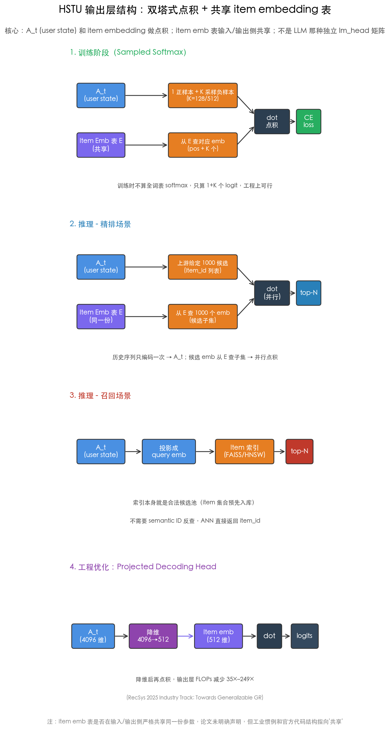
A key point to emphasize: HSTU’s output layer is not an independent \(W_{output}\) matrix like in LLMs, but a “two-tower dot product” structure — user state \(A_t\) and item embedding are dot-producted to get the score, and the item embedding table is shared between the input side (encoding history sequence) and the output side (scoring), with the same parameters. This is consistent with the scoring method of traditional two-tower recall models.
Similarity with traditional recall models
Speaking of this, you’ll find an interesting similarity: HSTU’s training paradigm is very similar to the traditional two-tower recall model — both do user embedding and item embedding dot product, both train with sampled softmax (positive + sampled negatives). Classic recall models like DSSM, YoutubeDNN, MIND all follow this pattern, and HSTU inherits this paradigm at the output layer and loss level.
The real difference is in the user encoder: traditional two-tower pools user historical behavior into a vector (mean/sum) or shallow MLP, while HSTU uses a sequence model to explicitly model dependencies between behaviors. So a more accurate statement is:
HSTU ≈ upgrades the two-tower recall’s user encoder from “pooling/shallow network” to “sequence model”, but retains the two-tower recall paradigm in training loss (sampled softmax) and scoring (dot product).
This also explains why HSTU can land in both fine-ranking and recall scenarios — its output layer structure is inherently two-tower dot product, naturally compatible with recall’s scoring method; and the user state quality improvement brought by sequence modeling lets it replace traditional fine-ranking. One model, two usages, behind which is the same training and scoring paradigm.
Change 2: Pointwise SiLU Replaces Softmax Attention
Motivation and attention basics
This change looks like just swapping an activation function, but what it really changes is the semantics of attention: standard softmax attention outputs “weighted average”, HSTU’s pointwise SiLU outputs “evidence accumulation”.
First explain what attention is doing. One-sentence summary: the position to be predicted emits a query \(Q\), going into history to find relevant information; each behavior in history has a “label” \(K\) and a “content” \(V\) (the information this behavior carries). \(Q\) dot-products with some \(K\) to get a “relevance score” — the larger the score, the more relevant this historical item is to the current query. Then aggregate all \(V\) by relevance scores to get attention’s output.
To get the numbers clear, we simplify vectors to 1-dim scalars (real models use multi-dim vectors, but 1-dim suffices to illustrate).
Suppose we want to predict “the user’s interest in the next basketball video”, so the query \(Q\) is “basketball direction”. There are two types of videos in history:
| Historical behavior | Type | \(K\) (label) | \(V\) (content) | Relevance score \(s = Q \cdot K\) |
|---|---|---|---|---|
| 1st | Basketball | 1.0 | 1.0 | 1.0 |
| 2nd | Basketball | 1.0 | 1.0 | 1.0 |
| 3rd | Basketball | 1.0 | 1.0 | 1.0 |
| 4th | Food | 0.1 | 0.2 | 0.1 |
That is, basketball videos all have relevance score 1.0 (strongly relevant), the food video’s relevance score is 0.1 (weakly relevant).
Now compare three users: user A has only 1 basketball history, user B is the table above (3 basketball + 1 food), user C has 100 basketball histories.
How softmax attention computes
Standard Transformer attention: first \(\exp\) each relevance score, then normalize into “weights summing to 1”, then use these weights to do weighted average over \(V\). The formula:
\[ A = \sum_j \mathrm{softmax}(s_j) \cdot V_j,\quad \mathrm{softmax}(s_j) = \frac{e^{s_j}}{\sum_k e^{s_k}} \]
User A (1 basketball):
- Scores: \([1.0]\)
- Normalized weights: \([1.0]\) (only one position, weight naturally 1)
- Output: \(1.0 \times 1.0 = \mathbf{1.0}\)
User B (3 basketball + 1 food):
- Scores: \([1.0, 1.0, 1.0, 0.1]\)
- After \(\exp\): \([2.72, 2.72, 2.72, 1.11]\)
- Sum: \(2.72 \times 3 + 1.11 = 9.27\)
- Normalized weights: \([0.294, 0.294, 0.294, 0.120]\)
- Output: \(0.294 \times 1.0 + 0.294 \times 1.0 + 0.294 \times 1.0 + 0.120 \times 0.2 = 0.882 + 0.024 = \mathbf{0.906}\)
Note what happens here: user B watched 2 more basketball videos than A, but the output actually drops from 1.0 to 0.906 — because the 3 new basketball videos have to compete for the same fixed weight budget of 1 with that food video, each basketball gets only 0.294, dragging the total weight down.
User C (100 basketball):
- All scores 1.0
- Normalized weights: each \(1/100\)
- Output: \(100 \times (1/100) \times 1.0 = \mathbf{1.0}\)
Putting the three results side by side:
| User | History | Softmax output |
|---|---|---|
| A | 1 basketball | 1.0 |
| B | 3 basketball + 1 food | 0.906 |
| C | 100 basketball | 1.0 |
The problem immediately surfaces: user A watched only 1 basketball, user C watched 100 — the interest strength clearly differs by 100×, but softmax gives almost identical outputs. Softmax can only express “what is the interest direction”, not “how strong is the interest”. The reason is the normalization: all weights are forced to sum to 1; whether there’s 1 or 1000 historical items, the total attention budget is fixed.
How pointwise SiLU attention computes
HSTU’s approach: don’t normalize; let each historical item independently contribute a piece of evidence, then just sum them. The formula:
\[ A_i = \sum_{j \le i} \mathrm{SiLU}(s_j) \cdot V_j,\quad \mathrm{SiLU}(x) = x \cdot \sigma(x) = \frac{x}{1 + e^{-x}} \]
Here \(\mathrm{SiLU}\) (also called swish) is an activation function whose shape is: larger input \(x\) → larger output; when input is small or negative, output approaches 0. It replaces softmax’s normalization but retains the role of “non-linear transformation on relevance scores”.
First compute two SiLU values we’ll need:
- \(\mathrm{SiLU}(1.0) = 1.0 \times \sigma(1.0) = 1.0 \times 0.731 = 0.731\)
- \(\mathrm{SiLU}(0.1) = 0.1 \times \sigma(0.1) = 0.1 \times 0.525 = 0.0525\)
User A (1 basketball):
- Output: \(\mathrm{SiLU}(1.0) \times 1.0 = 0.731 \times 1.0 = \mathbf{0.73}\)
User B (3 basketball + 1 food):
- Basketball contribution: \(3 \times \mathrm{SiLU}(1.0) \times 1.0 = 3 \times 0.731 = 2.193\)
- Food contribution: \(\mathrm{SiLU}(0.1) \times 0.2 = 0.0525 \times 0.2 = 0.0105\)
- Output: \(2.193 + 0.0105 = \mathbf{2.20}\)
User C (100 basketball):
- Output: \(100 \times \mathrm{SiLU}(1.0) \times 1.0 = 100 \times 0.731 = \mathbf{73.1}\)
Three results side by side:
| User | History | Softmax output | SiLU output |
|---|---|---|---|
| A | 1 basketball | 1.0 | 0.73 |
| B | 3 basketball + 1 food | 0.906 | 2.20 |
| C | 100 basketball | 1.0 | 73.1 |
The difference is clear:
- Under softmax, users A and C have almost identical outputs (1.0 vs 1.0), no strength difference visible
- Under SiLU, user C’s output is 100× user A’s (73.1 vs 0.73), directly reflecting the interest strength difference between “watched 100” and “watched 1”
This exactly corresponds to the signal recommendation cares most about — “how interested the user is in basketball” is itself hidden in the absolute count of “how many interactions”.
Restoring to the multi-dim vector form in real models
The above example simplified vectors to 1-dim scalars so you can follow along. In real models \(Q, K, V\) are multi-dim vectors, but the core logic is exactly the same. Let me first clarify a few transformer basics that are easily overlooked, so the formulas below are understandable.
First, \(Q, K, V\) are not directly trained parameters, but intermediate results after projection of the input. HSTU’s input at step \(t\) is an event vector \(x_t = \mathrm{Embed}(i_t, a_t, c_t, \Delta t_t, \dots)\) — it describes “what item the user interacted with at step \(t\), what action, in what scenario, how long since last”. Then three shared trainable weight matrices \(W_Q, W_K, W_V\) project \(x_t\) into three roles:
\[ q_t = W_q \tilde{x}_t,\quad k_t = W_k \tilde{x}_t,\quad v_t = W_v \tilde{x}_t \]
All positions in the sequence share the same \(W_Q, W_K, W_V\) — the difference is only in the input \(x_t\) (basketball event vs food event), so the projected \(K\) differs. The basketball video’s \(K=1.0\) and food video’s \(K=0.1\) in the example can be understood as “the learned \(W_K\) projects these two event types to different label positions”.
Second, what attention really does is aggregate historical events into “user state”. HSTU at step \(t\) uses attention to aggregate \(x_1, \dots, x_t\) into a hidden state \(A_t\) — this is “the user’s state after experiencing \(t\) steps of behavior”, while \(x_t\) itself is just the event at step \(t\). The whole sequence modeling is the cycle of “based on \(x_1, \dots, x_t\) compute state \(A_t\), then based on \(A_t\) predict what behavior is most likely at step \(t+1\)”.
With these two points understood, the difference between the two formulas becomes clear. Standard Transformer attention:
\[ A_i = \sum_{j \le i} \mathrm{softmax}(q_i^\top k_j) \cdot v_j,\quad \sum_j \alpha_{ij} = 1 \]
HSTU’s pointwise normalized-less attention:
\[ A_i = \sum_{j \le i} \phi(q_i^\top k_j + b_{ij}) \cdot v_j,\quad \phi = \mathrm{SiLU} \]
Symbol definitions:
- \(q_i, k_j, v_j\): query / key / value vectors, from positions \(i\) and \(j\) respectively (obtained by \(W_Q, W_K, W_V\) projection above)
- \(b_{ij}\): optional position / time / relative order bias, expressing the relationship between “how long ago a behavior happened” and “the current behavior”
- \(\phi\): activation function. HSTU uses SiLU (also called swish), no softmax normalization
- \(A_i\): the hidden state aggregated from historical behavior at position \(i\)
- \(j \le i\): causal mask, only allows the current position to see the past, not peek at the future
The two formulas differ only by a softmax, but their semantics are completely different: softmax outputs “weighted average”, SiLU outputs “evidence accumulation”. A rough analogy summarizes the difference:
- softmax attention is like asking: “Of these 100 historical items, which are most important? Distribute the total weight of 1 among them.”
- pointwise SiLU attention is like asking: “How much evidence can each historical item provide? Add the useful ones, add less or none for the useless ones.”
Why is this especially important for recommendation but not so much for NLP? This can actually be reverse-inferred from the precondition under which softmax normalization holds in NLP. Softmax normalizes weights to 1, essentially assuming “historical positions are in competition” — tokens in a sentence explain each other within a limited context, “which token is more important” is a reasonable question, and normalization lets the model focus on the most relevant few. But recommendation behavior sequences are completely different — repeat counts, continuous interactions, and interest strength themselves are features; behaviors shouldn’t compete for the same attention budget. HSTU switching to pointwise SiLU essentially acknowledges “in recommendation scenarios, the weighted average semantics reasonable in NLP is actually wrong, and should be replaced by evidence accumulation”. The HSTU paper observed on synthetic data that this difference can bring up to 44.7% NDCG gap.
Change 3: Retaining Hash / Sparse System, Not Strongly Dependent on Semantic ID
This point is exactly what was mentioned in change 1, and is also a point very easily misunderstood.
The TIGER / OneRec generative route is highly dependent on semantic ID — because they want to “generate items”, they must first turn items into generatable token sequences. A common misunderstanding is “since HSTU is a generative recommender, it should also depend on semantic ID”. But HSTU’s official implementation is exactly the opposite, mostly still using hash ID + sparse feature embedding.
Why can HSTU not depend on semantic ID?
Because HSTU challenges the parts of cascade’s assumptions B and C that it actually solves, not all of them. Specifically:
- Challenges B1 (pointwise independent scoring): HSTU uses sequence modeling to replace pointwise scoring — training objective changes from “per-sample classification” to “sequence transduction”, items are implicitly modeled through the history sequence, no longer isolated \((u, i)\) scoring
- Challenges C (no scaling law): HSTU uses pointwise SiLU attention + sequence transduction training objective + supporting engineering optimizations, making the recommender model follow power-law scaling over three orders of magnitude in compute, validating the recommender scaling law systematically for the first time
- Does not challenge A (item is discrete atom): in HSTU’s official implementation, items are still hash ID + sparse embedding, not replaced by semantic ID
- Does not challenge B2 (multi-step cascade approximates global optimum): HSTU still lands in the cascade system as fine-ranking or recall, not merging recall/ranking/reranking into one end-to-end model
The last point is easily misunderstood. “Generative” in the HSTU paper title refers to generative in modeling approach (reframing recommendation as next-action prediction), not generative in output form (autoregressively generating item tokens). The former is what HSTU does — using sequence modeling to replace independent scoring; the latter is what TIGER / OneRec do — decoding semantic ID token sequences and mapping back to real items. HSTU’s official implementation does not generate item tokens, so it still depends on ANN retrieval and still lands in the cascade system.
What really challenges B2 (end-to-end replacement of cascade) is OneRec — it uses an encoder-decoder to generate the whole list in one go, unifying recall + ranking + slate in one generative framework. This point will be clearer in the later “GR’s landing forms across cascade layers” comparison table: HSTU is in “first-layer fine-ranking”, OneRec is in “end-to-end”.
So the core of HSTU is “scalable sequence modeling on behavior sequences”, not “redesigning item representation”. Hash ID in HSTU is just one kind of action token — as long as behavior sequence modeling is strong enough, the model itself learns relationships between items, no need to switch to semantic ID.
HSTU and semantic ID are orthogonal
So HSTU and semantic ID are two orthogonal things:
- If the business’s main bottleneck is cold-start, long-tail, unstructured item representation, semantic ID is more direct — it gives new items a structured position
- If the business’s main bottleneck is behavior sequence modeling capability and model scaling, HSTU is more direct — it solves backbone capability, not item representation
- If both hold, in theory semantic ID can be fed to HSTU as part of item representation, but this is just icing on the cake, not a prerequisite for HSTU to hold
This point matters for actual deployment: no need to finish semantic ID before trying HSTU; the two can proceed independently.
Route 2: End-to-End Generative (OneRec / TIGER Family)
Route 1 is “train backbone on recommendation data but don’t generate item tokens” — HSTU lands in fine-ranking/recall, still a module in the cascade system. Route 2 is more radical: train an encoder-decoder from scratch on recommendation data, autoregressively generate item tokens (semantic IDs), unifying recall + ranking + slate in one generative framework, aiming to end-to-end replace cascade.
Representative works are OneRec (arXiv:2502.18965) and TIGER (arXiv:2305.05065). The two have similar architectural ideas, but very different deployment maturity — TIGER stopped at academic validation, OneRec has been deployed at scale on Kuaishou’s main app (full deployment data in OneRec Technical Report, arXiv:2506.13695).
OneRec’s core changes are as follows:
- Encoder-decoder structure: encoder processes user history sequence, decoder autoregressively generates the next (or next group of) item’s semantic ID tokens
- Session-wise list generation: not predicting item by item, but generating the whole session’s item list at once, letting the model learn the relative relationships and ordering among items
- Strong dependence on semantic ID: because it needs to “generate items”, it must first represent items as generatable token sequences (RQ-VAE semantic ID) — this contrasts with HSTU’s “no strong dependence on semantic ID”
- MoE parameter scaling: OneRec’s decoder FFN uses MoE, letting the model scale from 0.015B to 2.633B parameters while still following the scaling law
The figure below shows the core flow of end-to-end generative recommendation like OneRec:
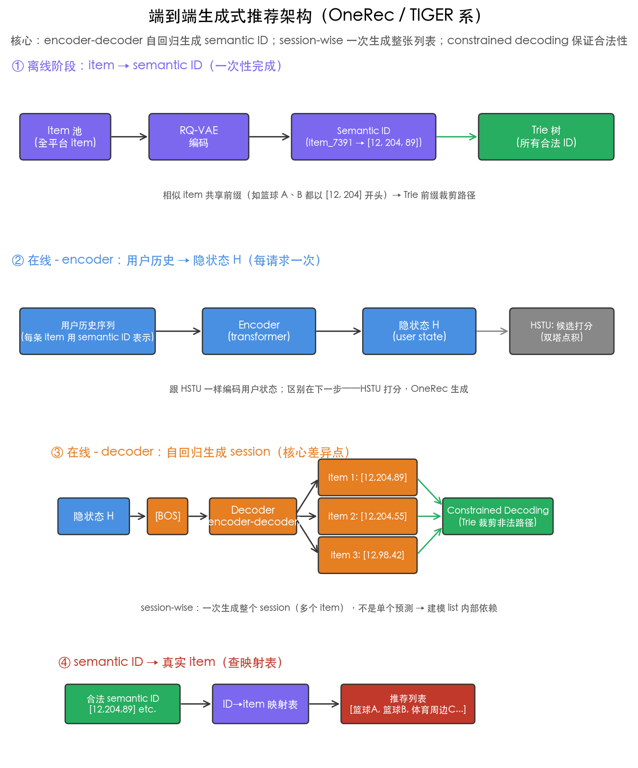
It’s divided into five steps (engineering details deferred to the later “Decoding & Inference” section):
- item → semantic ID (offline, one-time): each item is encoded into a semantic ID token sequence via RQ-VAE, similar items share prefixes. This step is the foundation for efficient path pruning in subsequent constrained decoding
- User history → encoder hidden state (online, once per request): user history sequence (each historical item also represented by semantic ID) is fed into the encoder to get hidden state \(H\). This step is the same as Route 1 HSTU encoding user state; the difference is the next step — HSTU uses \(H\) to score candidates, OneRec uses \(H\) to drive the decoder
- Decoder autoregressively generates semantic ID (session-wise): based on \(H\), starting with
[BOS], the decoder autoregressively generates a complete session (5-10 items) of semantic ID sequences. This is the key difference between Route 2 and Route 1 — HSTU’s candidates are given by upstream and it only scores; OneRec generates the whole list itself - Constrained decoding ensures validity: the decoder’s raw generated token sequence may not correspond to any real item; engineering uses Trie-based constrained decoding to ensure only valid semantic IDs are generated
- semantic ID → real item: valid semantic IDs are looked up back to real items via a mapping table, forming the final recommendation list in generation order
Training objective
Route 2’s training objective is next-token CE loss, corresponding to “given history and generated tokens, predict the next semantic ID token”:
\[ \mathcal{L}_{\text{NTP}} = -\sum_{i=1}^{m} \sum_{j=0}^{L-1} \log P(c^{(j)}_i \mid [\text{BOS}], c^{(1)}_1, \dots, c^{(j-1)}_i; \Theta) \]
Where \(m\) is the number of items in a session, \(L\) is the semantic ID layer count per item, \(c^{(j)}_i\) is the \(j\)-th codebook index of the \(i\)-th item. The generation probability of the whole session can be decomposed as (TIGER’s formula):
\[ P(\text{session} \mid \text{history}) = \prod_{i=1}^{m} \prod_{j=0}^{L-1} P(c^{(j)}_i \mid c^{(<j)}_i, \text{history}) \]
The alignment stage (IPA) does not only optimize DPO loss, but adds NTP loss and DPO loss weighted as a joint training objective (see the later “Training Objective: From next-token to preference alignment” section):
\[ \mathcal{L} = \mathcal{L}_{\text{NTP}} + \lambda \mathcal{L}_{\text{DPO}} \]
What’s most unique about Route 2 is not “generating items” itself (TIGER also generates items), but session-wise list generation — generating the whole session at once rather than one item at a time. This brings two benefits:
- Modeling relative relationships and order among items: traditional pointwise/next-item prediction can only ask “what is the next item”; session-wise can ask “what should this whole screen recommend, and in what order”, letting the model learn intra-list dependencies itself (e.g., recommending sports peripherals after a basketball video is more reasonable than recommending food)
- Naturally unifying recall + ranking + slate: the traditional cascade’s three steps “recall pulls candidates → fine-ranking scores → reranking produces slate” are compressed into one step “decoder generates the whole slate at once” in session-wise generation. This is the fundamental reason Route 2 can challenge assumption B2 (multi-step cascade approximates global optimum) — it directly replaces multi-step cascade with one-step generation
The latency challenge of autoregressively decoding the whole list is very severe — beam search, constrained decoding, KV cache, MoE sparse activation and other engineering optimizations are key to OneRec’s deployment. These engineering details are deferred to the later “Decoding & Inference” section, which will use OneRec as a concrete example to tie together constrained decoding, beam search, industrial latency constraints and other general mechanisms.
Route 1 and Route 2 both train from scratch on recommendation data, but their “output form” is completely different:
| Dimension | Route 1 (HSTU) | Route 2 (OneRec) |
|---|---|---|
| Generates item tokens | No (two-tower dot-product scoring) | Yes (autoregressively generates semantic ID) |
| Depends on semantic ID | Not strongly (hash ID works too) | Strongly (must generate tokens first) |
| Which cascade layer it lands in | Fine-ranking / recall (replaces one layer) | End-to-end (unifies recall + ranking + slate) |
| Challenged cascade assumptions | B1 (pointwise independent scoring) + C (scaling law) | B2 (multi-step cascade approximates global optimum) |
| Inference form | encode history once + score candidates in parallel | autoregressively decode the whole list |
| Candidate pool guarantee | Upstream-given / ANN index | constrained decoding + Trie pruning |
| Output per request | top-N candidate scores | a whole session list |
This difference determines the deployment difficulty of the two — HSTU lands in one cascade layer, can be progressively replaced in engineering; OneRec is an end-to-end replacement of cascade, with much larger engineering scope, but also a much higher ceiling.
OneRec is currently one of the most complete and typical industrial cases of end-to-end GR replacing cascade in public materials. The original paper OneRec (arXiv:2502.18965) only reported one deployment number — main-site watch-time +1.6%; more complete deployment data comes from the follow-up OneRec Technical Report (arXiv:2506.13695):
- Kuaishou main app + Lite version short video main scenarios: bears about 25% QPS; App Stay Time +0.54% main site, +1.24% Lite version (OneRec + RM Selection vs traditional cascade); LT7 +0.05% main site, +0.08% Lite version. The paper notes that at Kuaishou, a 0.1% App Stay Time improvement and 0.01% LT7 improvement already counts as statistically significant
- Local life services scenario: GMV +21.01%, order volume +17.89%, paying users +18.58%, new customer acquisition efficiency +23.02%, already 100% QPS fully switched (OneLoc series work, see arXiv:2508.14646)
- Operating cost (OPEX) is only 10.6% of the traditional solution
But Route 2 also has its limitations:
- Independent validation still limited: OneRec / OneLoc / OneRec V2 all come from the Kuaishou technical lineage; public materials already cover short video, local life and other scenarios, but still lack same-level end-to-end validation from a second company in main recommendation scenarios. In contrast, Route 1 (HSTU) has Meta (HSTU multi-product deployment) + Meituan MTGR (arXiv:2505.18654, MTGR-large fully deployed on Meituan take-away recommendation main traffic) — two independent deployments.
- Large refactoring scope: end-to-end replacement of cascade means the entire recall/ranking/reranking chain must be refactored, much larger than HSTU replacing one layer.
- Inference latency challenge: autoregressively decoding the whole list is inherently disadvantageous; OneRec V2’s Lazy Decoder-Only architecture is the latest engineering progress in this direction.
OneRec’s detailed RL alignment method (Iterative Preference Alignment) will be expanded separately later; here we only discuss its position among the three routes.
Route 3: Directly Reusing General LLMs
The core thesis of this route: general LLMs have already learned rich world knowledge and text understanding capability; just rewrite recommendation as a prompt / instruction task — no need to train a recommendation foundation model from scratch.
Looking at three representative works in chronological order reveals the evolution logic of “letting LLMs do recommendation”: from initially “let the LLM generate everything”, gradually retreating to “let the LLM only do fine-ranking scoring” — each retreat was forced by the real constraints of recommendation scenarios.
P5 (RecSys 2022, arXiv:2203.13366): the earliest full-textualization attempt
P5’s idea is “fully language-ize recommendation” — based on T5 encoder-decoder (223M parameters), all recommendation data (user-item interactions, user descriptions, item metadata, reviews) is turned into text prompts, then pre-trained with a shared language modeling objective on multiple tasks. P5 unified five task types:
- Rating prediction: predict rating for a user-item pair
- Sequential recommendation: predict next item given a historical interaction sequence
- Explanation generation: generate recommendation rationale text
- Review summarization: summarize long reviews into titles
- Review preference prediction: predict rating from reviews
P5’s most critical design choice: item IDs are split into sub-word tokens — e.g., item_7391 is tokenized into item, _, 7391 three sub-words. This means items can be autoregressively generated by the decoder, exactly like an LLM generating natural language. P5’s pitch is “one model, multi-task + zero-shot generalization” — after pre-training it can generalize to unseen prompts and new items.
But P5 has an obvious problem: item IDs are generated as text tokens, with no mechanism to ensure the generated ID falls in the valid item pool. The model might generate a non-existent item_99999, or an ID that’s semantically reasonable but not in the pool. This is the inevitable cost of treating recommendation as NLP — the LLM’s vocabulary is open, but the recommendation scenario’s item pool is closed.
BIGRec (arXiv:2308.08434): acknowledging that generation results need grounding
BIGRec proposed a bi-step grounding paradigm for P5’s “generated ID invalid” problem:
- Step 1 (grounding): fine-tune the LLM to generate item-description-related tokens, “grounding” the LLM from language space to recommendation space
- Step 2 (matching): use the LLM’s latent representation to map generated tokens to the closest valid item
That is, BIGRec no longer expects the LLM’s generated token sequence itself to be a valid item ID, but treats it as a “semantic anchor”, then uses nearest-neighbor search to map back to the valid item pool. This is similar in spirit to “the output layer is two-tower dot product + ANN retrieval” in the HSTU route — both acknowledge the generation side can’t directly guarantee validity and need post-processing mapping.
But the BIGRec paper also reveals a deeper finding: the pure LLM route’s efficiency and stability in learning collaborative signals is still insufficient. The paper observed that increasing the number of training samples brings limited marginal gains for BIGRec — because the LLM’s strong semantic prior suppresses learning of statistical information (e.g., popularity, collaborative filtering signals). This point is key to the overall judgment of Route 3: what the LLM learns in pre-training is “semantic associations in language”, not “collaborative associations in user behavior” — the former is semantic signal, the latter is statistical signal, and the two are not equivalent.
LlamaRec (PGAI@CIKM 2023, arXiv:2311.02089): just give up generating items, let the LLM only do fine-ranking
LlamaRec’s idea: since LLM item generation has validity and efficiency issues, then simply don’t let the LLM generate items, only let it do fine-ranking scoring. Specifically two stages:
- Stage 1 (recall): use a traditional sequence model (SASRec/LRURec) for recall, pulling back a candidate item set
- Stage 2 (fine-ranking): feed user history and candidate items as text to the LLM, use a verbalizer to directly map LLM output logits to a probability distribution over candidate items
The key is the verbalizer trick — mapping each candidate item to a specific token (or set of tokens) in the LLM’s vocabulary, so one forward pass reads out all candidates’ logits, no autoregressive generation needed. LlamaRec uses LLaMA-2-7b + LoRA fine-tuning; the verbalizer lets it complete all candidate scoring in one forward pass, bypassing the slowness of LLM autoregressive decoding.
This design is clever: it changes the LLM’s output layer from “generator” to “scorer” — the LLM no longer generates items, just uses its semantic understanding capability to score candidate items. This is similar in spirit to HSTU’s “output layer is two-tower dot product”: both “use the model to encode a query/user state, then score candidate items”; HSTU’s backbone is a sequence model, LlamaRec’s backbone is an LLM.
The evolution logic reflected by the three papers
Putting the three together, Route 3’s evolution direction is very clear:
| Paper | Year | LLM’s role | How item validity is guaranteed |
|---|---|---|---|
| P5 | 2022 | Generate item ID | Not guaranteed (generated tokens may not be a valid ID) |
| BIGRec | 2023 | Generate item description tokens | Post-processing mapping (latent nearest neighbor) |
| LlamaRec | 2023 | Score candidate items | Candidates given by upstream (LLM not responsible for generation) |
The evolution direction is: from “let the LLM generate items” gradually retreating to “let the LLM score”. Each retreat was forced by real constraints of recommendation scenarios:
- P5 doesn’t guarantee validity → BIGRec adds grounding post-processing
- BIGRec’s grounding is still slow (generation + mapping), and the pure LLM route is inefficient at learning collaborative signals → LlamaRec just gives up generation, only does scoring
- Finally LlamaRec retreats to the “LLM does fine-ranking” position — overlapping with HSTU’s position in the fine-ranking scenario, but with the backbone swapped to an LLM
This evolution also explains why Route 3 currently has little industrial deployment — retreating to LlamaRec’s slot, the LLM’s advantage over traditional fine-ranking is only “semantic understanding capability”, but it’s at a disadvantage in inference latency, behavioral signal modeling, and training cost. The LLM’s semantic understanding capability has local value in “long-tail, cold-start, conversational” sub-scenarios, but in main recommendation scenarios with “huge behavioral data, strict latency requirements”, this advantage is insufficient to overcome latency and cost disadvantages.
Two industrial extension works: HLLM and URM
P5/BIGRec/LlamaRec are all academic works, but Route 3 has two industrial extensions worth mentioning separately — both “use LLM ideas for recommendation”, but took a different path from pure LLM-as-Recommender:
- HLLM (ByteDance, arXiv:2409.12740): uses two layers of LLM to decouple “item content understanding” and “user behavior modeling” — the Item LLM compresses item text descriptions into content embeddings, the User LLM does behavior modeling on these embeddings. This decoupling is especially suitable for scenarios with “rich item content information, relatively sparse behavioral signals” (e.g., long videos, e-commerce products), with very significant improvements on cold-start and long-tail — these scenarios are exactly where the LLM’s semantic understanding capability can truly play its value
- URM (Alibaba, arXiv:2502.03041): treats recall as a “universal task” — the same model can do multi-scenario recall, multi-objective recall, and long-tail recall. Multi-query representation lets the model produce multiple query embeddings in one inference, each query corresponding to a different objective / scenario. This is essentially porting the LLM’s “instruction-following” idea to recommendation recall
The common feature of these two works: they don’t let the LLM directly generate item tokens, but use LLM ideas to transform some internal module of the recommender system. This is much easier to deploy industrially than P5’s “fully language-ize recommendation” route — and is one of the few directions in Route 3 with public industrial A/B or testing evidence.
Differences Among the Three Routes
Many interpretations treat HSTU, OneRec, LLM-as-Recommender as “similar things”, but looking closely, their starting points, what they reuse, and what scenarios they suit are all completely different:
| Dimension | Route 1 (HSTU) | Route 2 (OneRec) | Route 3 (LLM-as-Recommender) |
|---|---|---|---|
| Starting point | Train from scratch on recommendation data | Train encoder-decoder from scratch on recommendation data | Fine-tune from pre-trained LLM |
| What it reuses | Scaling law itself | Scaling law + semantic ID + end-to-end | LLM’s world knowledge + text understanding |
| Generates item tokens | No (two-tower dot-product scoring) | Yes (autoregressively generates semantic ID) | Partially generates (P5/BIGRec), partially scores (LlamaRec) |
| Key signal | Behavior sequence | Behavior sequence + item representation structure | Text description |
| Challenged assumptions | B1 (pointwise) + C (scaling law) | B2 (multi-step cascade) + C (scaling law) | Mainly B1 (LLM replaces scoring) |
| Suitable scenarios | Feed / short video with huge behavioral data | End-to-end unifying recall + ranking + slate | Long-tail, cold-start, conversational |
| Inference latency | Medium (specialized architecture can be deeply optimized) | High (autoregressively decode whole list) | High (general LLM decode slow) |
| Industrial deployment evidence | Meta (HSTU multi-product deployment) + Meituan MTGR (arXiv:2505.18654) | Kuaishou main app + Lite version deployment | Almost none in main scenarios, some in local scenarios |
| Deployment difficulty | High, but validated feasible by Meta | Very high, large engineering scope | High, very few industrial cases |
| Industrial evidence strength | Validated (paradigm-level contribution) | End-to-end evidence relatively complete, but mainly from one technical lineage | Academically valid, industrially unvalidated |
| Main bottleneck | No obvious bottleneck; Meta (HSTU) + Meituan (MTGR) two independent big-company validations | Large refactoring scope, severe inference latency, public evidence mainly from one technical lineage | Insufficient behavioral signal injection + inference latency hard to compress to tens of milliseconds; only long-tail/cold-start/conversational has local value |
Decoding & Inference: Letting Generated Tokens Land on Real Items
Core question: the generated token sequence may not correspond to any real item at all
A token sequence sampled from an autoregressive model can be any natural language in a normal LLM scenario. But in GR, the generated semantic ID must be mappable back to a real, currently valid, currently unblocked item. Otherwise the recommendation result is just air.
Engineering has several standard approaches to this problem. Below we use OneRec as a concrete example to tie this mechanism together — TIGER’s mechanism is essentially the same, just not deployed industrially.
Beam search: avoid greedily discarding high-probability paths too early
The most basic approach. Greedy decode picks the highest-probability token each step, but semantic ID is a multi-token sequence — some path may have high first-step probability but no way forward next step (remaining tokens all invalid), and greedy gets stuck. Beam search simultaneously maintains top-k candidate paths and expands them in parallel, finally picking the highest-total-probability complete path.
OneRec’s beam size is on the order of 128 — meaning each step must maintain 128 paths’ KV cache and probabilities simultaneously, putting pressure on both memory and bandwidth. This number directly determines the latency floor of decoding.
Constrained / prefix-aware decoding: doing softmax only on the valid set
Beam search solves “which path to pick”; constrained decoding solves “at each step, only do softmax on valid tokens”. At each decode step, first mask out all invalid tokens, then do softmax and sample, eliminating the generation of air items at the source.
The hierarchical structure of semantic IDs makes this step naturally fit a Trie:
- Layer-1 tokens can only be chosen from “layer-1 codebook indices that appeared in the training set”
- Layer-2 tokens can only be chosen from “layer-2 combinations that appeared in the training set given the layer-1 token”
- And so on
That is, the prefix of a semantic ID alone can prune most invalid paths. OneRec pre-organizes all valid semantic IDs into a Trie; during decoding, each step advances one node on the Trie, and the next step’s valid token set is exactly this node’s child key set — one mask operation completes the constraint.
This point is a key engineering trick used by both TIGER and OneRec, and is the engineering reason for Route 2’s “strong dependence on semantic ID” — without RQ-VAE encoding items into hierarchical-prefix semantic IDs, constrained decoding degenerates into masking all item IDs, losing the prefix-pruning efficiency advantage.
Relationship with ANN
There’s a common misunderstanding to clarify: GR’s generative recall is not “replacing ANN”; a more accurate statement is “using transformer memory to replace the ANN index”. That is, recall becomes “the model parameters themselves are the index”, not “model + external index”. This distinction matters engineering-wise: model retraining means index retraining, model deployment means index deployment, the two can no longer be deployed independently.
Industrial latency constraints: the biggest bottleneck of autoregressive decoding
Traditional fine-ranking finishes in tens of milliseconds industrially; autoregressive decoding is inherently disadvantaged — each token requires one forward pass. Generating a session of 5-10 items, each with 3-4 layers of semantic ID tokens, totals 15-40 forward passes, plus beam size 128 parallel expansion — naive implementation’s latency is completely unusable.
OneRec’s deployment relies on several engineering optimizations stacked to bring latency down:
- KV cache: reuse encoder hidden states and K/V of already-generated tokens, avoiding recomputing history each step
- MoE sparse activation: decoder FFN uses MoE; each token activates only a few experts, actual compute much less than a dense model — this lets the model scale to 2.6B parameters while still following the scaling law, without single-step latency exploding
- float16 / low-precision inference: further compress memory and bandwidth
OneRec V2 (arXiv:2508.20900)‘s Lazy Decoder-Only architecture claims to reduce total compute by 94%, training resources by 90%, and scale the model to 8B parameters — the latest engineering progress in this direction. Its core idea is to delay some tokens’ decoding, only running the full decoder when truly needed, reducing wasted computation.
Constrained decoding and transformer-as-index themselves have been validated as feasible by multiple industrial systems. But compared to the mature ANN + fine-ranking chain under the cascade paradigm, the latency overhead of autoregressive decoding remains significantly higher. This is why end-to-end GR has so far mainly deployed in “latency-relatively-lenient” content feed scenarios, while search and advertising — extremely latency-sensitive — have essentially none.
Training Objective: From next-token to Preference Alignment
The “generative architecture” discussed in the three pillars above uses next-token cross-entropy training. But this loss can only optimize “the next item the user is most likely to interact with” — this is just a surrogate, not the real target recommendation cares about. This section separately discusses alignment mechanisms beyond next-token loss.
Why next-token Loss Alone Is Insufficient
Four classes of problems next-token loss doesn’t solve:
- Multi-objective trade-off: trade-offs among CTR, watch-time, conversion, retention; next-token can’t explicitly express these
- Long-term value: session depth, next-day retention, repurchase — these signals are inherently delayed and sparse
- Business constraints: ad load, marketing-feel dispersion, category diversity — these hard constraints are outside the generative model’s view
- exploration: the model has only seen token combinations in historical logs, with no exploration motive for unseen combinations
In the LLM domain, the corresponding solution is RLHF (Reinforcement Learning from Human Feedback). GR inherits the idea of RLHF, but with several key differences from LLM. It needs to be pointed out up front that RL alignment can only solve soft-preference problems (multi-objective implicit trade-offs, long-term value, exploration); as for “business constraints” — pacing, load caps, score shading, calibration and other hard constraints and online control problems — the next-token paradigm is inherently unsuited, and RL can’t solve them either; traditional control methods are still needed as fallback (see the later “GR’s landing forms across cascade layers” section on the second-layer mix-rank discussion).
OneRec’s Iterative Preference Alignment
OneRec (arXiv:2502.18965) is currently the most representative industrial RL alignment solution in GR. Its approach has five steps:
Step 1: train a reward model \(R_\phi\)
Input is a session-level generated sequence (i.e., a list of items recommended to the user), output is a scalar reward. The reward’s training labels come from multi-objective business results — watch-time, engagement, conversion and other real metrics.
Step 2: use the current policy to generate candidate sessions
Use the current GR model (policy \(\pi_\theta\)) to generate \(K\) candidate sessions \(\{\pi^{(1)}, \dots, \pi^{(K)}\}\) via beam search. Here \(\pi\) denotes a complete recommendation session (not the \(\pi\) in the math symbol \(\pi_\theta\)); context will distinguish clearly.
Step 3: construct preference pairs
Use the reward model \(R_\phi\) to score each candidate; the highest-reward one is chosen (\(\pi^+\)), the lowest-reward one is rejected (\(\pi^-\)).
Step 4: NTP + DPO joint alignment
OneRec in the IPA stage does not only use DPO loss, but adds next-token loss and DPO loss weighted as a joint training objective:
\[ \mathcal{L} = \mathcal{L}_{\mathrm{NTP}} + \lambda \mathcal{L}_{\mathrm{DPO}} \]
Where the DPO loss’s specific form is:
\[ \mathcal{L}_{\mathrm{DPO}} = -\,\mathbb{E}\left[\log \sigma\!\left(\beta \log \frac{\pi_\theta(\pi^+)}{\pi_{\mathrm{ref}}(\pi^+)} - \beta \log \frac{\pi_\theta(\pi^-)}{\pi_{\mathrm{ref}}(\pi^-)}\right)\right] \]
Symbol definitions:
- \(\pi_\theta\): current policy (GR model)
- \(\pi_{\mathrm{ref}}\): reference policy — in OneRec this is the previous iteration’s model \(M_t\) (not a frozen SFT-stage checkpoint), updated each iteration
- \(\pi^+, \pi^-\): high / low reward candidate sessions
- \(\beta\): temperature coefficient, controlling alignment strength. Larger \(\beta\) → policy more tightly follows preference; smaller \(\beta\) → policy more conservative
- \(\sigma\): sigmoid function
- \(\lambda\): DPO loss weight. In the paper, DPO samples are about 1% of NTP samples; \(\lambda\) balances the magnitudes of the two losses
Two key points to emphasize here:
- NTP loss always retained: even in the IPA stage, next-token loss is not dropped — it’s trained jointly with DPO loss as a combined loss, serving as an anchor preventing the policy from drifting too far. If only DPO loss is kept and NTP loss dropped, the policy will quickly be led astray by the reward model’s bias
- Reference policy is dynamic: unlike LLM RLHF’s practice of “freezing the SFT checkpoint as reference”, OneRec’s \(\pi_{\mathrm{ref}}\) is the previous iteration’s model \(M_t\), updated each iteration — this is another meaning of “iterative”
In plain terms, this joint loss wants to: make the policy’s relative probability of outputting \(\pi^+\) higher than \(\pi^-\) (DPO part), while not drifting too far from the reference policy (\(\beta\) term), and still doing well on next-token prediction (NTP part).
Step 5: iterate
After jointly training with \(\mathcal{L} = \mathcal{L}_{\mathrm{NTP}} + \lambda \mathcal{L}_{\mathrm{DPO}}\) to get \(M_{t+1}\), use \(M_{t+1}\) as the new policy to regenerate candidates, re-score with the reward model, reconstruct preference pairs, and jointly train \(M_{t+2}\). In each iteration, NTP loss participates in training together with DPO loss, not dropped when switching to the alignment stage. This iterative process is the source of “Iterative Preference Alignment” in OneRec’s name.
Summarizing the whole training flow: first train a seed model with pure NTP loss (SFT stage) → enter the IPA stage, where each iteration jointly trains with \(\mathcal{L}_{\mathrm{NTP}} + \lambda \mathcal{L}_{\mathrm{DPO}}\), with the reference policy being the previous iteration’s model (dynamically changing).
The Essential Difference Between GR’s RL and LLM’s RLHF
Comparing OneRec with LLM’s RLHF, the most critical difference is the source of preference pairs:
In LLM’s RLHF, preference pairs are obtained by human annotators comparing item by item. NLP’s output space is natural language, with controllable annotation cost.
In GR, no one wants to compare recommendation lists item by item — each recommendation is several to dozens of items, annotating one session takes minutes, doesn’t scale. So GR’s preference pairs are synthesized from a reward model: the reward model itself simulates user behavior and generates preferences itself.
The cost of this is very large. It means GR’s RL alignment essentially becomes “model-based RL on a learned simulator” — the simulator’s (reward model’s) own bias is a new source of risk. If the reward model is learned inaccurately, the whole alignment runs in the wrong direction. This point isn’t specifically emphasized in the OneRec paper, but is a pit that must be stepped on industrially.
It needs to be further pointed out that the reward model itself is also trained from historical user behavior logs — its training labels are usually a weighted combination of watch-time, engagement, conversion and other business metrics. This means the reward model learns “the preference distribution that has appeared in historical logs”, with no judgment for unseen item combinations. So GR + RL alignment essentially bears two layers of bias: (1) the reward model’s bias as a simulator, (2) the bias in the reward model’s training labels (multi-objective weighting + historical log coverage). The second layer of bias is the same problem as traditional multi-objective recommendation modeling, but because GR relies on the reward model to synthesize preferences, this bias gets amplified by DPO.
GR’s Landing Forms Across Cascade Layers
This section is an explicit echo of the previous article 《Personalized Ranking Formula》 — mapping the GR paradigm layer by layer back to cascade, to see which layer is overturned, which is reopened, and which remains unsolved.
The previous article divided recommendation into three layers:
- First layer fine-ranking: single item scoring \(s(u,i,x)\)
- Second layer mixed ranking: business-level traffic allocation, online control with constraints
- Third layer re-ranking: list combination optimization, including listwise / Slate
Adding recall, cascade is actually four layers. GR’s corresponding form across these four layers is completely different, as summarized below:
| Cascade stage | Traditional approach | GR corresponding form | Representative work | Industrial deployment |
|---|---|---|---|---|
| Recall | Two-tower + ANN | TIGER: generative recall (transformer memory replaces ANN); HSTU: sequence modeling + ANN (user encoder upgrade, item side unchanged) | TIGER / HSTU | TIGER academically valid, industrial-scale recall unvalidated; HSTU High (Meta deployment) |
| First-layer fine-ranking | pointwise / multi-objective weighted | Autoregressive Ranking | HSTU | High (Meta deployment) |
| Third-layer re-ranking / Slate | listwise + Generator-Evaluator | Directly generate slate | OneRec, Seq2Slate family | Medium (Kuaishou deployment) |
| Second-layer mixed ranking (business allocation) | calibration + multiplier + pacing + score shading | Hard constraints / online control — GR doesn’t solve currently | — | Low |
The first three layers’ details on TIGER / HSTU / OneRec have been covered in the three pillars above; here we only point out their correspondence to cascade layers. Among them, GR on the recall side actually has two different routes (TIGER generative recall vs HSTU sequence-modeling recall) that need to be examined separately. What this section really wants to say is the last row — the hard constraints and online control part of the second-layer mixed ranking is a blind spot that the next-token paradigm is inherently unsuited for and GR currently can’t well satisfy, expanded separately at the end.
Recall
Traditional recall uses user/item two-tower learning of embeddings, builds ANN index offline, and does approximate nearest-neighbor retrieval online. GR on the recall side actually has two different routes, corresponding to the two kinds of works discussed above:
HSTU route: sequence-modeling recall — doesn’t generate item tokens, just upgrades the user-side encoder in the two-tower to HSTU sequence model, projects a stronger user state \(A_t\) into a query embedding, then feeds it to the ANN index for retrieval; the item side is still hash ID + embedding + ANN (see the earlier Route 1 HSTU output layer discussion). This route retains the engineering advantage of ANN index being independently deployable and updatable, but sacrifices the ability to “generalize to unseen items”.
TIGER route: generative recall — given a historical behavior sequence, autoregressively generates the next item’s semantic ID (see the earlier Item Tokenization section). The most essential difference between this and two-tower recall is not “a different retrieval method”, but gives the recall side for the first time the ability to generalize to unseen items. In two-tower recall, items not in the training set can hardly be recalled; in GR recall, as long as the new item’s semantic ID falls in the learned prefix space, it may be generated. The cost is that transformer memory itself is the index; model retraining means index retraining, and the two can no longer be deployed independently (see the earlier “Relationship with ANN” section).
Two levels need to be distinguished — recall task and industrial-scale recall — TIGER has only been validated at the first level:
- Recall task level (validated): the TIGER paper indeed does recall-task experiments — given user history, generate the next item’s semantic ID, then do constrained decoding to map back to real items. This itself is the form of a recall task; the paper title “Generative Retrieval” also clearly positions TIGER as generative recall.
- Industrial-scale recall level (unvalidated): TIGER’s benchmarks are academic datasets like Amazon Reviews, with SOTA comparisons mainly against sequence-recommendation models like SASRec / BERT4Rec, not two-tower recall models; it also didn’t experiment in industrial recall scenarios with million/billion-scale item pools + ANN indexes. So “vs two-tower + ANN” is more a paradigm-level comparison (transformer memory replaces ANN index), not a conclusion directly drawn from the paper’s experiments.
This two-level distinction is the root cause of TIGER’s “opens new possibilities” but relatively weak industrial deployment evidence — it proved on academic benchmarks that generative recall as a task is feasible, but whether industrial-scale recall can outperform the mature “two-tower + ANN” chain has no public evidence yet.
The industrial deployment of these two routes differs greatly: the TIGER route has only been validated on academic benchmarks (e.g., Amazon Reviews, comparing against sequence-recommendation models like SASRec / BERT4Rec) for the feasibility of generative recall as a task itself, with no experiments in industrial recall scenarios with million/billion-scale item pools + ANN indexes, and no public deployment evidence; the HSTU route comes with traffic naturally as HSTU deploys across multiple Meta products. In other words, the GR form that has actually been deployed industrially on the recall side is HSTU’s “sequence modeling + ANN” route, not TIGER’s “fully generative” route — the latter is more like “a direction opening new possibilities”, the former is “a validated deployment form”.
First-Layer Fine-Ranking
HSTU is the most fundamental challenge to cascade’s first layer — no longer pointwise scoring, but next-action sequence prediction (reframing recommendation from “per-\((u,i)\) scoring” to “given a historical behavior sequence, predict what behavior is most likely next”). No longer making “multi-objective weighting” central, but using scaling law + large model capacity to automatically learn implicit trade-offs among multi-objectives (see the earlier Route 1).
The only point to emphasize here, distinct from the three pillars above: HSTU challenges the mathematical form “first-layer scoring formula \(f_\theta(u,i,x)\)” from the previous article itself, not item representation. HSTU doesn’t use semantic ID; the official implementation is mostly still hash-based — meaning even a team that doesn’t plan to switch to semantic ID can independently try HSTU. This point is the root cause of the difference in deployability between fine-ranking and recall layers in GR.
Third-Layer Re-Ranking / Slate
OneRec (arXiv:2502.18965) uses an encoder-decoder to generate the whole list in one go, the most natural evolution of the third layer in the previous article.
The previous article divided third-layer methods into three classes: constrained re-ranking, list re-ranking, Slate optimization. The most common industrial implementation of “list re-ranking” is Generator-Evaluator: the generator produces multiple candidate arrangements, the evaluator scores each arrangement’s overall utility. OneRec unifies these two things in one transformer:
- The decoder is both generator (autoregressively generates arrangements) and implicitly serves as evaluator via next-token loss
- Training uses RQ-VAE semantic ID to represent items, making “adjacent items” also adjacent in token space
- Uses DPO for preference alignment (see the earlier “Training Objective: From next-token to preference alignment” section)
That is, OneRec unifies listwise and Slate in one generative framework, as the “next-generation form” of the previous article’s third layer.
Second-Layer Mixed Ranking: Hard Constraints and Online Control Are GR’s Current Blind Spot
This is the most important paragraph in this section, and also the most easily overlooked.
In the previous article, the second-layer mixed ranking does “multi-business, constraint-bearing traffic allocation”: calibration, multiplier, pacing, score shading, minimum traffic protection, ad load caps… these problems need to be distinguished into two classes:
- Soft-preference class (implicit trade-offs among multi-objectives, user preference alignment) — this part can be put into the GR framework, learned via DPO / reward alignment (see the earlier “Training Objective: From next-token to preference alignment” section)
- Hard-constraint + online-control class (pacing, load caps, score shading, calibration) — this part is a blind spot that the next-token paradigm is inherently unsuited for and GR currently can’t well satisfy
The common feature of the latter class: they’re not “predict the next token” problems, but “online control under constrained resource conditions” problems.
The next-token paradigm is inherently unsuited to express this class of problems:
- Pacing controllers need long-time-window feedback accumulation; next-token loss is stepwise
- Load constraints are hard constraints, not soft preferences; DPO-style reward alignment is unsuited to express them
- Score shading is essentially an online estimation of a dual variable (shadow price), more like a control theory problem than a generation problem
- Each business’s calibration magnitude alignment is also not solvable by “generation”
So even if a team fully switches to GR, the hard constraints and online control part of the business-level mixed ranking layer (second layer) still need to retain traditional methods. This is a very important but rarely paper-discussed fact about GR industrial deployment.
Overall, GR is disruptive for the first layer (HSTU), opens new possibilities for recall — TIGER’s fully generative recall is “the direction of new possibilities”, HSTU’s “sequence modeling + ANN” is “the validated deployment form”, and is unifying for the third layer (OneRec); the soft-preference part of the second-layer mixed ranking can be put into the GR framework, but the hard-constraint and online-control part (pacing / load / score shading / calibration) the next-token paradigm is inherently unsuited for, and traditional methods must be retained.
Practical Feasibility Judgment
This section consolidates the judgments scattered throughout the article into an actionable checklist. To judge whether GR is feasible for a specific business, the key is not “whether it’s hype overall”, but to break it into several independent technical points — each with different industrial evidence strength. Below we first go through the evidence point by point, then land on “what business should try now” and “how to try”.
| Technical point | Industrial evidence | Main basis |
|---|---|---|
| Semantic ID / RQ-VAE | Validated | TIGER experiments sufficient; OneRec, HLLM all depend on it; prerequisite for the “generate item token” route |
| HSTU + recommender scaling law | Validated (strongest) | Meta 1.5T-parameter deployment |
| End-to-end GR replacing cascade | Short video / local life has public validation, independent validation still limited | OneRec / OneLoc / OneRec V2 etc. Kuaishou technical lineage cases are relatively complete, but cross-company validation insufficient |
| LLM-as-Recommender (P5 / BIGRec / LlamaRec) | Academically valid, industrially unvalidated | Benchmarks look good; two fundamental problems — latency and behavioral signal injection — unsolved |
| GR + DPO preference alignment | Short video validated, sparse reward unsolved | OneRec effective on watch-time; sparse-reward scenarios unsolved |
| GR for cold start | Strong evidence | semantic ID + content encoder naturally carries semantic structure; HLLM long-tail experimental evidence |
| GR replacing business-level mixed ranking | GR alone cannot replace | pacing / load / calibration still need external controllers and traditional online control mechanisms |
| GR inference latency | Still a bottleneck | OneRec V2 cutting 94% compute is progress, but still higher than cascade |
If a business simultaneously meets multiple of the following, trying GR is worthwhile:
- Behavioral data volume large enough: scaling law can take effect. A rough empirical threshold is hundred-million-DAU, billion-level daily interactions
- Main feedback dense and timely: short video watch-time, feed dwell time — this dense reward is the prerequisite for GR + RL alignment to work
- Strong need for item content understanding / cold start: content platforms, UGC platforms, cross-domain recommendation
- Recall is clearly a bottleneck: two-tower recall ceiling obvious, long-tail coverage poor — then generative retrieval is the most direct entry point for gains
- High list-combination quality demand with relatively single objective: feed scenario slate generation benefits most
Conversely, if a business has any of the following characteristics, then in the short term GR is not recommended as the main direction:
- Strong constraints, strong multi-objective: advertising, e-commerce scenarios simultaneously managing load, pacing, calibration, revenue. GR can learn some soft preferences, but can hardly bear these hard constraints and online control alone
- Inference latency extremely sensitive: search, ad RTB with tens-of-millisecond budgets
- Business data scale not large enough: scaling law can’t kick in, instead dragged down by the general architecture
- Main feedback sparse and delayed: scenarios where long retention, repurchase, conversion are the main objectives
If deciding to proceed with GR, a relatively robust path is phased:
- First deploy semantic ID, gradually replacing hash ID. This step, even without full GR, can yield cold-start and long-tail gains
- On the recall side, do a generative retrieval pilot, parallel small-traffic validation with the existing two-tower recall
- On the fine-ranking side, try HSTU-style scaling experiments, first seeing whether scaling law really holds on your business — this is the key decision point for follow-up investment
- After 1-3 are all validated, then consider slate generation + DPO alignment
- Business-level mixed ranking layer (constrained allocation) retains traditional methods; don’t try to replace everything with GR
The logic behind this path: each step retains retreat room, each step’s ROI can be independently evaluated. Compared to directly “end-to-end deploy GR”, industrial risk is much lower.
Summary
Returning to the title’s question: what GR replaces is not the cascade system form itself, but part of the modeling assumptions behind cascade.
It first replaces the assumption that “items are just unstructured IDs”. Semantic ID / RQ-VAE turns an item from a hash key into a token with hierarchical structure, which is key for cold-start, long-tail, and generative recall. But this mainly serves the TIGER / OneRec “generate item token” route, and is not a prerequisite for all GR forms.
It also replaces part of the assumption that “each item can be scored independently”. HSTU pushes recommendation from pointwise scoring to behavior sequence modeling, and demonstrates the recommender model’s scaling law at large-scale compute; OneRec goes further, compressing recall, ranking, and slate generation into one end-to-end generative framework. Both are called GR, but their engineering meaning is completely different: HSTU is more like a strong backbone in the cascade system, OneRec is what challenges the overall cascade chain.
But GR does not replace business-level mixed ranking and online control. Pacing, load, calibration, score shading — these problems are essentially constrained resource allocation, not next-token prediction. GR can learn soft preferences and partial multi-objective trade-offs, but hard constraints still need external controllers and traditional mechanisms as fallback.
So the more accurate judgment is: GR is not the end of cascade, but reopens several key links in the recommender system. The industrial evidence for semantic ID and HSTU is already fairly strong; end-to-end GR, represented by the OneRec technical lineage, has public validation in short video and local life scenarios, but cross-company independent validation is still limited; LLM-as-Recommender in the main recommendation chain is still more like local augmentation, with value mainly in long-tail, cold-start, content understanding, and conversational scenarios.
If a business has huge behavioral data, dense timely feedback, and relatively single constraints, GR is worth systematic investment; if the business is extremely latency-sensitive, has many hard constraints, and sparse delayed rewards, GR is more suitable as a local module experiment, not a direct replacement of the whole cascade.
References
- Understanding Scaling Laws for Recommendation Models (Ardalani et al., arXiv:2208.08489)
- Recommender Systems with Generative Retrieval (TIGER, NeurIPS 2023)
- Actions Speak Louder than Words: Trillion-Parameter Sequential Transducers for Generative Recommendations (HSTU, ICML 2024)
- OneRec: Unifying Retrieve and Rank with Generative Recommender and Iterative Preference Alignment
- OneRec Technical Report
- OneRec-V2 Technical Report
- OneLoc: Geo-Aware Generative Recommender Systems for Local Life Services
- HLLM: Enhancing Sequential Recommendations via Hierarchical Large Language Models for Item and User Modeling
- Large Language Models Are Universal Recommendation Learners (URM)
- P5: Recommendation as Language Processing
- LlamaRec: Two-Stage Recommendation using Large Language Models for Ranking
- BIGRec: A Bi-Step Grounding Paradigm for LLMs in Recommendation
- MTGR: Industrial-Scale Generative Recommendation Framework in Meituan (KDD 2025)
- Personalized Ranking Formula: From Personalized Fine-Ranking to Personalized Mixed-Ranking to Global Re-Ranking (previous article on this blog)