Personalized Ranking Formulas: From Item Scoring to Mixed Ranking to Global Reranking
The “personalized ranking formula” is a recurring topic in recommendation systems, but the term itself is often imprecise — we tend to lump together three fundamentally different problems.
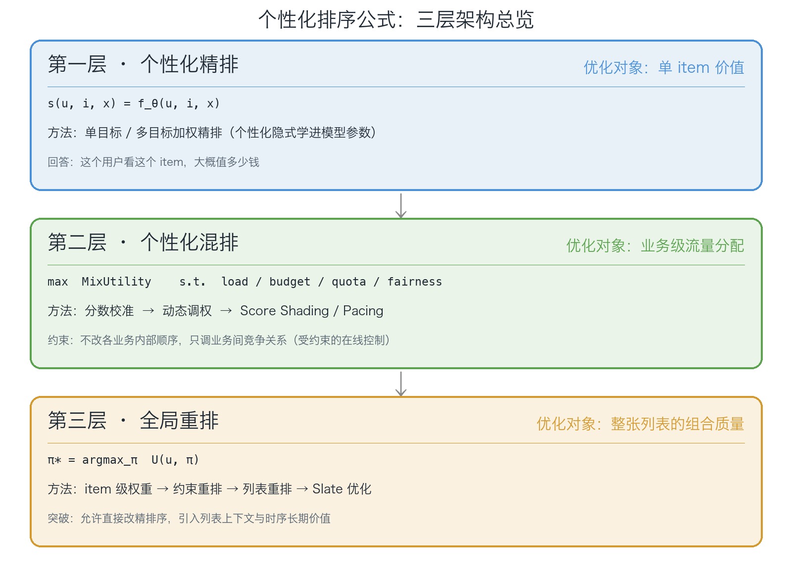
More precisely, personalized ranking in a recommendation system typically involves at least three layers:
- Layer 1: Personalized scoring (fine ranking), which answers “what is the value of showing this item to this user?”
- Layer 2: Personalized mixed ranking (blending), which answers “when multiple business lines compete for the same impression slot, who should get it?”
- Layer 3: Global reranking, which answers “the user sees an entire list — how should we assemble it?”
For many modern recommendation systems, Layer 1 is already strong enough.
User embeddings, item embeddings, multi-task learning, cross features — all of these aim at the same target: getting the model to accurately predict how valuable a (user, item) pair is. In that sense, most production rankers are already personalized; that personalization just isn’t written as “one set of weights per user” — it’s been absorbed implicitly into the model parameters.
Yet real systems exhibit something that looks contradictory at first glance: even with a strong Layer 1, production still runs Layer 2 blending, traffic control, quota management, plus Layer 3 reranking, and additionally bolts on score calibration, pacing, shading, and listwise reranking.
The intuitive explanation is: “Layer 1 isn’t accurate enough, so Layer 2 and Layer 3 are patches.” That isn’t entirely wrong, but it’s only half the story.
The deeper reason is that Layer 1, Layer 2, and Layer 3 are not optimizing the same thing.
- Layer 1 optimizes per-item value prediction
- Layer 2 optimizes constrained traffic allocation across business lines
- Layer 3 optimizes overall list composition
For this reason, the truly interesting question about “personalized ranking formulas” is not “why are different users’ weights different” but rather: once Layer 1 can already reasonably learn a user’s per-item preferences, why does the platform still need Layer 2 mixed ranking and Layer 3 global reranking? What is each layer compensating for, and what is each layer optimizing?
This article is about exactly that three-layer question.
Before diving into the details, here is a one-shot overview of what each layer optimizes, its key methods, and where its boundary lies:
What Layer 1 solves
Mathematically, Layer 1 learns a scoring function:
\[ s(u,i,x) = f_\theta(u,i,x) \]
where \(s(u,i,x)\) is the score / predicted value produced by Layer 1, \(f_\theta\) is a scoring function with parameters \(\theta\); \(u\) is the user, \(i\) is the item, \(x\) is the context, and \(\theta\) are the model parameters. This score essentially answers:
Given the current context, what value do we expect from showing this item to this user?
This value can be a single objective such as CTR, or a combination of multiple objectives:
\[ s(u,i,x) = w_1 \cdot CTR + w_2 \cdot CVR + w_3 \cdot WatchTime + w_4 \cdot GMV \]
Here \(w_1, w_2, w_3, w_4\) are the fusion weights across objectives; CTR, CVR, WatchTime, and GMV stand for click-through rate, conversion rate, watch time, and gross merchandise value respectively.
A sufficiently strong model can pick up deep personalization differences:
- Some users prefer longer dwell time
- Some users are more easily converted by e-commerce content
- Some users are highly ad-averse
- Some new users need stable experiences; some heavy users tolerate more aggressive personalization
So, for the question “is this user a match for this item,” Layer 1 already does a lot. What it’s really good at, in one sentence:
Roughly how much is this item worth to this user.
The catch is that recommendation systems were never solving only that one question.
Why per-item scoring isn’t enough
If we wanted to do everything with just Layer 1, we’d need at least four conditions (assumptions) to hold at the same time.
These four conditions split into two groups:
- Per-item additivity and score commensurability together determine whether the “sum-then-sort” pointwise paradigm is mathematically valid at all — they are the root reason Layer 3 (list-level combinatorial optimization) exists
- No additional global constraints and a static environment together determine whether the problem still carries resource constraints and a time dimension — they are the root reason Layer 2 (traffic allocation and online control) exists
Per-item additivity
The overall utility of the final list must satisfy:
\[ U(\pi) = \sum_{k=1}^{K} v(u, i_{\pi_k}, k) \]
Here \(U(\pi)\) is the total utility of permutation \(\pi\) (we suppress its dependence on user and context for brevity). \(K\) is the list length, \(i_{\pi_k}\) is the item at position \(k\), and \(v(u, i_{\pi_k}, k)\) is the per-item value at position \(k\) for user \(u\). This formula already encodes a strong assumption: each item’s value depends only on the user, the item itself, and its position — not on the other items in the list.
But in real systems this assumption is often broken. The more common form is:
\[ U(\pi) = \sum_{k=1}^{K} v(u, i_{\pi_k}, k) + \sum_{k<l} g(i_{\pi_k}, i_{\pi_l}, u) \]
where the second term \(g(i_{\pi_k}, i_{\pi_l}, u)\) captures the additional interaction effect of two items co-appearing in the same list — complementarity, substitution, fatigue, or diversity gain. For example:
- Two highly similar videos shown back-to-back: the second one is much less engaging
- Too much of the same kind of content in a row: users get fatigued faster
- Interleaving articles, short videos, and live streams: users typically stay engaged longer than with a single format
- Different positions suit different content — eye-catching items work at the top, follow-on content works further down
- When users look at an entire page, they perceive not just per-item quality but also how varied and fresh the page is, and how well it matches their current context
Once this interaction term exists, pointwise per-item scoring is no longer sufficient to derive the optimal final list.
Score commensurability
This condition is also almost never satisfied in practice.
Scores from different business lines, different models, and different objectives typically don’t share a common scale:
- 0.4 from the article ranker
- 0.2 from the live-streaming ranker
- An eCPM from ads
- A GMV estimate from e-commerce
These scores come from different training objectives, sample distributions, noise levels, and business semantics. Even if they all “look like a number,” that doesn’t mean they can be directly compared.
So Layer 1 can’t fully nail down per-item value, and multi-objective scores can’t easily be made commensurable — both are important reasons why Layers 2 and 3 exist.
But that’s not the whole story.
No additional global constraints
If the only goal were to maximize a single unified utility, Layer 1 alone really could do most of the work.
But real recommendation systems usually come with many constraints that act on the overall result:
- Load constraints from monetization-style business lines (ads, e-commerce, live streaming) — these are really LT-based but often expressed as load
- Marketing-mix de-clustering (e.g., no two consecutive monetization items)
- Diversity
- Author / merchant fairness
- Platform ecosystem balance
- …
These constraints don’t act on any single item; they act on the entire list, the entire time window, or even the entire traffic pool. So no matter how accurate a single item’s score is, that alone doesn’t satisfy these constraints automatically.
A static environment
If the traffic environment were static, ranking would be much simpler.
But real systems live in a continuously changing dynamic environment:
- Has a particular business line already over-served this hour?
- Has the user already grown tired?
- Should we preserve some exploration traffic right now?
- Has supply of a certain content type suddenly dropped?
By this point the problem is no longer just “ranking” — it’s a dynamic decision problem with a strong flavor of control.
So a real recommendation system is not solving a static “score each item then sort” problem. It’s solving a dynamic systems problem: allocating traffic under constraints, assembling lists, and keeping the system stable.
That is why, even with a strong Layer 1, Layers 2 and 3 cannot be omitted.
Layer 2’s responsibility: allocating traffic across business lines
In many recommendation systems, the entities competing for impressions are not a single content source but multiple business lines competing for the same impression slot:
- Articles
- Short videos
- Live streams
- E-commerce cards
- Ads
- Local life content
Each business line typically has its own retrieval, pre-ranking, and ranking pipeline, each capable of answering “within my queue, which item is best.” But the question the platform really needs to answer is not “which item is best within this business” — it’s “for this specific impression slot, which business line should win?”
This is no longer a per-item value-prediction problem. It’s a classic cross-business resource allocation problem.
And this problem usually comes with a stack of platform constraints by default:
- Some business has a penetration target
- Some business’s load cannot drop too far
- Ads must stay below a cap
- The platform doesn’t want any single content type to crowd out the others long-term
- Some business’s user experience is already strained
- Some business has limited server or supply capacity at the moment
- Some business’s ranker scores don’t translate directly to a head-to-head comparison with another business
At this point, the problem the platform really faces looks more like the following, where \(\text{MixUtility}\) is the overall utility the blending layer wants to maximize, and \(\text{Load}, \text{Budget}, \text{Quota}, \text{Risk}, \text{Fairness}\) are platform constraints on traffic share, budget, quota, risk, and fairness:
\[ \begin{aligned} \max \quad & \text{MixUtility} \\ \text{s.t.} \quad & \text{Load},\text{Budget},\text{Quota},\text{Risk},\text{Fairness} \end{aligned} \]
At this point, no matter how well Layer 1 predicts per-item value, it cannot answer “how should traffic be allocated” on its own.
The platform still needs an additional decision layer to handle:
- How to calibrate scores across business lines
- Given current budget and targets, which business line is the better recipient of this impression
- Whether a given business should bid up, bid down, hold supply, or limit supply
- How to balance local utility against system-wide stability
That is the reason Layer 2 (mixed ranking / blending) exists.
A concrete example:
Suppose a user clearly prefers live streams over articles. The most natural reaction is to globally bump up the weight on live streams in the blending layer.
This often works, because it’s solving exactly the right question: should this impression come from the live-streaming queue or the article queue?
But there is a boundary that must be made explicit: Layer 2 can only decide “who gets the traffic”; it cannot decide “which item within that business should be served.”
If the top-1 inside the live-streaming queue happens to be a hard-sell live commerce stream while the user actually likes “casual knowledge-sharing live streams,” then no matter how much the blending layer boosts the live-stream weight, all it does is repeatedly push the wrong kind of live stream at the user. So while Layer 2 is necessary, it has a natural ceiling: it is more like a business-level scheduler than a per-item selector.
Treating each business as an already-sorted queue, what Layer 2 does becomes very intuitive:
- Don’t change the internal order of any queue
- For each slot, decide which queue to pull the next card from
In other words, Layer 2 doesn’t optimize per item; it optimizes a business-level / source-level traffic scheduling policy.
A common misconception: isn’t Layer 2 essentially each participant adjusting its own weights so everyone’s scores end up commensurable?
That’s only half the answer.
Layer 2 does include “making different business lines’ scores roughly comparable,” but that’s only the starting point, not the whole of it. More completely, Layer 2 does two things:
- First, map each participant’s local value into a roughly competitive shared space
- Then, on that shared space, do constrained dynamic traffic allocation given platform constraints, budget state, and traffic targets
So score commensurability is more like Layer 2’s entry ticket, while constrained resource allocation is the actual main problem of Layer 2.
From this angle, all of the following methods sit in Layer 2:
- Score calibration
- Personalized multiplier
- Quota / pacing
- Score-shading / bid-shading-style dynamic score adjustment
- Various constrained order-preserving blending schemes
So Layer 2 isn’t just patching up “inaccurate ranker scores.” It adds a new layer of capability to the platform:
Constrained, dynamic, personalized traffic control on top of the existing per-business rankers, without touching their internal order.
Layer 2’s methods: personalized mixed ranking that preserves per-business order
We’ve covered why Layer 2 must exist. Now let’s look at how — what its mainstream methods actually are.
Score calibration
This is the most overlooked, yet most engineering-critical, step.
Scores from different business lines are rarely on the same scale:
- 0.4 from the article ranker
- 0.2 from the live-streaming ranker
- 15 from ad eCPM
- Some normalized value of GMV from e-commerce
Comparing these scores directly is usually meaningless, because their underlying model objectives, sample distributions, training procedures, and business semantics all differ.
So before any real personalized blending, the platform usually does a calibration step, including:
- Bucketed calibration
- Quantile normalization
- Platt scaling / isotonic regression
- Conditional calibration by user segment or scene
Or, in the simplest case, just pick a fixed coefficient per business from average scale ratios over a recent window. The essence of this step is: first solve “can we even compare these,” then solve “how to divide them up.”
Without calibration, the downstream personalized multipliers, pacing, and shading will all be distorted.
Dynamic weighting
Once different business lines’ scores are roughly comparable, the most direct approach is to apply a dynamic weight at the business level:
\[ \text{MixScore}_{u,b} = \alpha_{u,b}(x) \cdot \text{CalibScore}_b \]
where:
- \(\text{MixScore}_{u,b}\) is the mixed-ranking score for user \(u\) and business \(b\) on the current request
- \(\text{CalibScore}_b\) is the calibrated comparable base score for business \(b\)
- \(b\) indexes business / source
- \(\alpha_{u,b}(x)\) is user \(u\)’s preference weight for business \(b\) under context \(x\)
For example:
- Users who prefer live streams get a higher multiplier on the live-stream source
- Users who prefer articles get a higher article multiplier
- Some contexts favor short videos, some favor e-commerce cards
This approach is simple, intuitive, interpretable, and fits naturally on top of any existing multi-business stack. It is fundamentally order-preserving blending — it only adjusts inter-business competitiveness without changing intra-business order.
But its ceiling is just as clear: it can only answer “who gets this traffic,” not “which item within that business should be served.”
Score Shading / Pacing: viewing blending as constrained dynamic bidding
Going one step further, platforms realize that user preference weights alone are not enough — many problems aren’t really about “preference” but about “in the current constraint state, is this traffic slot worth winning?”
A natural framing here is to view a business’s blending score as an implicit bid.
If bid shading in ads solves:
In a first-price auction, how do we cut cost and lift ROI without losing the ability to win volume?
then score shading in blending solves:
Without changing intra-business order, how do we dynamically adjust a business’s PK score to find a better balance among penetration, cost, and stability?
For a given business, the problem can be written as:
\[ \begin{aligned} \max_{s_i} \quad & \sum_i V_i F(s_i) \\ \text{s.t.} \quad & \frac{1}{n}\sum_i s_i F(s_i)\le C \end{aligned} \]
where:
- \(V_i\): the value this business gets if it wins opportunity \(i\)
- \(s_i\): this business’s blending score / PK score on opportunity \(i\)
- \(F(s_i)\): the win rate at score \(s_i\)
- \(n\): the number of opportunities / samples in the statistics window
- \(C\): the cost or scale constraint
By Lagrangian duality, this can be turned into a per-request decision problem:
\[ s_i^\star = \arg\max_{s_i} F(s_i) \left( V_i - \lambda s_i \right) \]
Here \(\lambda\) is strictly the Lagrange multiplier on the cost constraint (i.e., a shadow price); in production it is typically tracked online by a pacing controller (PID/EMA, etc.) such that the long-run average cost stays close to \(C\). \(s_i^\star\) is the optimal blending / PK score for opportunity \(i\).
This formula is representative because it makes one thing concrete: Layer 2 is not “fixing an inaccurate score” — it is solving a constrained online-control problem.
The hardest step in this method isn’t the formula itself but the win-rate model \(F(s)\). Intuitively, two routes:
- Point estimate: directly model \(P(\text{win}=1|s,\text{context})\), the probability of winning given score \(s\) and context
- Distribution estimate: don’t model the win rate directly; instead model the distribution of competitors’ top score, then derive the win rate from that distribution
The former is more intuitive; the latter is more complete.
A representative work here is Deep Landscape Forecasting for Real-time Bidding Advertising. Instead of learning “will I win at this bid,” it learns the competition landscape’s distribution parameters, from which the win rate at any bid can be derived analytically. The same idea transfers cleanly to blending: if you really want score shading to work, you often need not “win/no-win at this score” but “what does the entire competitive environment look like right now.”
Score shading is great for efficiency, but without governance it easily turns local optimization into global risk.
If every business is allowed to shade on its own, two failure modes show up quickly:
(1) Score deflation
Every business tries to “win with a lower score.” Over time, the system’s absolute score range drifts leftward, eventually breaking any strategy that depends on absolute-value thresholds.
(2) Control oscillation
When multiple businesses simultaneously run their own PID / pacing controllers, they all interact in the same shared traffic pool and form coupled oscillations. The most common symptom: one minute live streams take too much volume, the next minute short videos over-compensate, and the whole platform develops high-frequency jitter.
So in production, score shading is not just a modeling problem; it’s a platform-mechanism problem. At least one of the following governance strategies is usually needed:
- Global anchor: tie the system to a relatively stable value baseline
- Unified accounting mechanism: competition is judged not just by “who reports a higher score” but by “who actually contributes more global value”
For more details on Score Shading, see: From Bid Shading to Score Shading: Modeling, Control, and Game Dynamics in Mixed Ranking Optimization
Layer 3’s responsibility: assembling the entire list
If Layer 2 is mainly solving “who gets the traffic,” Layer 3 is solving a more fundamental problem: the user doesn’t consume a single item; the user consumes an entire list.
In Layer 2, the system mostly answers: which business / source gets this slot first. Its core objects are inter-business competition and traffic allocation; even with quota, pacing, and load constraints, what gets solved is usually business-level, time-window-level, or resource-share-level.
In Layer 3, the question shifts. The system now has to answer: how do we actually assemble the final list shown to the user?
That is the most fundamental difference between Layer 2 and Layer 3: Layer 2 decides “who gets the volume first,” while Layer 3 decides “what this list itself looks like.” The former manages inter-source competition; the latter directly faces top-k ordering, positions, context, and combinatorial quality.
That sentence sounds ordinary, but it implies something important: per-item optimality is not the same as list optimality.
Layer 1’s default logic is usually: higher score, higher rank. That logic implicitly assumes: total list value = simple sum of per-item values.
In reality, that assumption is often violated.
The clearest example is content fatigue. Suppose a user’s top-4 candidates are scored:
- Video A: 0.90
- Video B: 0.88
- Video C: 0.87
- Article D: 0.80
Sorting by score puts three very similar videos in a row. Each item alone looks great, but the combination might not. Swapping the third for Article D could yield a better overall page satisfaction.
This shows: even with very accurate per-item scoring, greedy pointwise sorting does not guarantee a globally optimal top-k list.
This is the root reason Layer 3 exists.
It no longer solves “what is this item worth”; it solves: how should this list be assembled so the overall result is best?
Layer 3’s methods: global reranking that may directly change the per-item order
In Layer 3, the optimization object is no longer “which business wins this impression” but the entire permutation:
\[ \pi^\star=\arg\max_{\pi} U(u,\pi) \]
where \(U(u,\pi)\) is the total utility of permutation \(\pi\) for user \(u\); \(\pi\) is the final list, and \(\pi^\star\) is the list that maximizes the objective.
What the system actually cares about here:
- top-k overall experience
- Item-item substitution and complementarity
- Diversity
- Position bias
- Fairness
- Long-term value
So this layer’s methods are significantly more complex than Layer 2’s. Before diving in, here is a high-level map. Layer 3 contains at least two steps:
- Define each item’s utility more reasonably. Item-level personalized weights live here; they answer “how much is this single piece of content worth”
- Optimize the final list more reasonably. Constrained reranking, listwise reranking, and slate optimization live here; they answer “given these items, how should the list be put together”
By analogy, item-level personalized weights are like deciding “what each brick is worth”; the other three are like deciding “how to lay these bricks into a wall.”
Continuing this decomposition, the second step further splits into three classes, from “hard rules” to “soft quality” to “temporal long-term value”:
- Constrained reranking: first answers “which lists must not be served”
- Listwise reranking: then answers “among the lists that can be served, which is best”
- Slate optimization: further answers “this list not only affects the current page but continues to shape downstream user behavior”
Each is covered below.
Item-level personalized weights
A boundary note first: strictly speaking, item-level personalized weights sit on the boundary between Layer 1 and Layer 3. We put them in Layer 3 here because only when they exist as “an extra utility-adjustment step after the ranker” do they belong to Layer 3; if folded directly into the ranker, they remain Layer 1. The discussion below assumes the former.
The most common — and most easily productionized — method here directly models item-level utility:
\[ U(u,i,x) = \sum_k w_k(u, x)\,\phi_k(i, x) \]
where:
- \(U(u,i,x)\) is the utility of item \(i\) to user \(u\) under context \(x\)
- \(\phi_k(i,x)\) is item \(i\)’s signal or predicted value on the \(k\)-th objective under context \(x\) — CTR, CVR, GMV, dwell time, retention, business value, etc.
- \(w_k(u,x)\) is a dynamic weight that depends on user and context
- \(k\) indexes the different objectives
Formally, this looks similar to Layer 2’s business multiplier — both are “weight × score” — but they act on completely different objects: Layer 2’s multiplier acts on the source / business level and decides “which business gets this traffic,” with intra-business order unchanged; the weight here acts on the item level and decides “what this single item is worth,” so it can directly change the order among items.
The deeper point this method is making: when multi-objective trade-offs vary with user and scene, the system can either absorb that variation implicitly into one shared scoring function, or expose it explicitly as item-level dynamic weights. As long as the model has enough capacity and the features cover user state and context, a shared parameter set can in principle learn the “weekday commute vs. weekend evening” difference too.
If we use one black-box model, we can still write \(U(u,i,x)=f_\theta(u,i,x)\); the personalized multi-objective trade-off is hidden inside the black-box utility function. If we write \(U(u,i,x)=\sum_k w_k(u,x)\phi_k(i,x)\), the system is explicitly modeling “do we currently care more about CTR, GMV, dwell time, or retention?”
In plain terms: this is not really about “can a single set of parameters do this” — it’s about “should the internal yardstick stay fixed across different users and different moments?” For example:
- For a high-spend user, GMV / CVR within a commerce content piece may matter more; for a casual entertainment user, dwell time, completion, and low-cost enjoyment may matter more
- For new users, the system may weigh retention, stable experience, and low intrusion more heavily; for heavy users, it may push more aggressive personalization, clicks, and conversion
- Even the same user has different value weights for weekday commute, weekday evening, and weekend leisure: sometimes more efficiency-driven, sometimes more relaxation-driven, sometimes more purchase-driven
So the value of explicit dynamic weights is often not “a black-box can’t do it” but that they offer stronger controllability, interpretability, and engineering decomposability.
There are many ways to learn these weights. In industry, three common families: supervised end-to-end fusion, contextual bandit, and actor-critic. They appear to learn the same weight function \(w_k(u, x)\), but they actually answer three different questions:
| Method | What question it answers | Feedback structure | Models “action affects future”? | Optimization target |
|---|---|---|---|---|
| Supervised end-to-end fusion | From historical logs, which \(w_k\) produces the best final list metric? | (context, label) static pair | No | Offline loss (proxy of the final metric) |
| Contextual Bandit | For this impression, which \(w_k\) gives the highest single-step reward? And how to explore new combinations? | (context, action, reward) single-step | No | Single-step immediate reward |
| Actor-Critic | This action affects user’s future state — which \(w_k\) maximizes long-term cumulative reward? | \((s, a, r, s')\) sequence | Yes | \(\sum_t \gamma^t r_t\) |
In plain terms:
- Supervised end-to-end is like looking at the answer sheet after the test: take a year of logs as training data and let the model directly approximate the “final metric.” Simple and stable, but it can only interpolate within the observed data distribution — any \(w_k\) combination not in the logs is a blind spot
- Contextual Bandit is like guessing which die is best before each roll, and immediately adjusting after seeing the result. The key difference from supervised: it actively explores. The key difference from RL: it assumes each decision is independent, ignoring how the current action shifts the next request’s user state
- Actor-Critic treats recommendation as an MDP: the current choice changes downstream user behavior; the Critic estimates “how much reward we can still collect starting from this state,” and back-propagates that signal into the Actor. The substantive new ingredient is acknowledging that actions change the future, at the cost of needing a stable dense-reward signal and dealing with high variance and distribution drift
In practice, these three are not substitutes; production stacks frequently layer them together: a supervised model learns a baseline \(w_k\); a contextual bandit explores on a small slice of traffic; an actor-critic optimizes longer-horizon, cumulative goals (LTV, session retention) — without replacing the immediate-reward target the supervised model already learns.
Below we zoom in on actor-critic’s actual industrial profile — the most controversial and most easily misrepresented of the three.
A fairly common practice is to use Actor-Critic / DDPG to directly learn \(w_k(u, x)\): the Actor outputs the multi-objective weights for \((u, x)\), the Critic evaluates the overall utility of the current impression / list, and the reward is set to watch time, completion rate, interaction signals, etc.
In short-video and live-streaming products — where feedback is dense and immediate — this pipeline really does work: every impression delivers dense reward, return signals are fast, the Critic actually learns, and the Actor receives a stable gradient. Kuaishou, ByteDance, Alibaba, and other content / e-commerce platforms all have public or semi-public practice along these lines. But for RL to land at this step, at least two prerequisites must hold:
- Reward must be dense enough and timely enough: watch time, completion, dwell are available on every impression with clear attribution. If switched to conversion, retention, repeat purchase (sparse, delayed signals), off-policy evaluation and attribution stability both degrade fast
- The Critic actually has to learn the list / impression-level utility: otherwise the Actor’s weights easily over-optimize a single metric (e.g., dwell time inflated, interaction sacrificed), breaking multi-objective balance
If the business’s primary feedback is itself sparse or delayed (clicks-to-conversion in e-commerce, long-horizon retention, etc.), then supervised end-to-end fusion or rule + segment-based weights is still the more cost-effective choice; contextual bandit sits in between and works well as an online-exploration supplement.
The next three sections move to the second step — “given these items, how do we put them together.”
Constrained reranking
In many businesses, the platform doesn’t merely “hope” certain conditions hold; it must enforce them. For example:
- Upper bound on ad load
- Minimum exposure for certain author types
- Upper bound on risky content
- Per-business quota
- Category-coverage requirements
This layer is necessary precisely because Layer 2, while handling some constraints at the business level, never actually solves “can this specific page be served the way it’s currently laid out?”
For example, if the platform requires top-10 to have at most 2 ads, no same-author content back-to-back, and at least 1 slot reserved for a certain content type, then:
- Layer 1 might give all 3 ads very high scores
- Layer 2 might already keep the ad business’s overall traffic within budget
- But on a particular request and a particular top-k, the system can still violate the rules
So why is it that this layer can change the order produced by earlier layers? Not because it has some mysterious new feature, but because it pushes constraints that earlier layers only handled at coarse business / time-window granularity down to the single-request, final-list level to be solved explicitly.
In other words, the incremental information constrained reranking actually receives is not “this item has one more feature” but rather “what’s already in this list, how many slots are left, and which constraints are close to being violated.” That information is only complete at the list-assembly stage.
Simple penalty or multiplier terms are usually not enough here: they only “lean” the result and can’t reliably guarantee a constraint holds. Too small, the constraint slips; too large, you crush overall relevance. Worse, many constraints are discrete, position-dependent, and tightly coupled — naturally not expressible as smooth additions to a single score.
A more natural formulation is:
\[ \begin{aligned} \max_{\pi} \quad & U(\pi) \\ \text{s.t.} \quad & C_j(\pi) \le 0 \end{aligned} \]
where \(C_j(\pi)\) measures how much permutation \(\pi\) violates the \(j\)-th constraint; \(C_j(\pi) \le 0\) means the constraint is satisfied.
The core idea of constrained reranking is not “tweak the score a bit more” but explicitly recognize: the final ranking is not a pure relevance-maximization problem but a combinatorial optimization problem with hard constraints.
Industry practice ranges from rule-aware greedy / swap, to more explicit constraint solvers like Lagrangian relaxation, min-cost flow, or ILP. The form varies; the essence is the same.
So what constrained reranking really fills in is the “last mile” that earlier layers don’t solve: not which item is worth more, not which business should get the volume, but whether the final list shown to the user can look good while still satisfying the boundaries the platform must hold.
Listwise reranking
Even when every hard constraint is satisfied, the story isn’t over: a list being “legal” doesn’t mean it’s a “good list.”
That’s exactly why listwise reranking exists: constrained reranking answers “which lists must not be served”; listwise reranking answers “among the legal lists, which is best.”
If we continue the previous logic, this layer can also change the per-item order only because it gains incremental information that earlier layers don’t have. Here that information isn’t mainly “are hard constraints satisfied” but what happens when items are placed together.
The real unsolved problem from earlier layers is item-item interaction and the overall quality of the list. Layer 1 and item-level dynamic weights are still scoring single items; Layer 2 handles inter-business traffic allocation; constrained reranking handles whether the result satisfies rules. Even with all of those done right, the system can still produce a list where “every item is decent, but together they don’t quite work.”
For example:
- Five items are all relevant and compliant, but they’re highly similar — running them together causes fatigue
- Two items each look fine alone, but once the first one satisfies the user’s intent, the second’s marginal value drops sharply
- The same set of items in positions 1–2 vs. positions 5–6 can produce a totally different user experience
- Some combinations break no rules but are clearly worse in pacing, richness, or sense of exploration
The point is: an item’s true value is no longer “independent of the other items.” The incremental information listwise reranking gains is often things like “context relationships,” “neighboring substitution and complementarity,” “position’s effect on satisfaction,” “how monotonic or how varied the current list is” — list-level context. These features aren’t necessarily invisible to the ranker, but they’re often not explicitly modeled and not explicitly optimized during the ranking stage.
These problems are also hard to write out completely as a set of hard rules, because “what makes a list better” tends to be a soft, holistic, context-dependent question.
Traditional pointwise / pairwise learning-to-rank focuses on single items or item pairs; listwise methods take the entire list as the optimization object directly.
From RankNet to LambdaRank to LambdaMART: An Overview systematically lays out the differences among pointwise, pairwise, and listwise. In recommendation reranking, the idea is pushed further:
If the user consumes the final list, the training objective should be as close to “final list quality” as possible, not just a single pointwise surrogate.
A representative work is Personalized Re-ranking for Recommendation. It applies stronger sequence modeling / self-attention on top of an existing candidate list to model item-item global relations, achieving personalized list-level reranking.
Strictly speaking, “listwise methods” come in two industrial flavors. Both take a list as input, but their outputs are quite different:
| Type | Input | Output | Typical use |
|---|---|---|---|
| Listwise scorer / context model | Candidate list | A new score per position (then argsort) | PRM-style contextual re-scoring |
| Listwise evaluator | A full permutation \(\pi\) | A scalar \(V_\phi(\pi)\) — the list’s overall utility | Generator-Evaluator paradigm |
The former implicitly assumes: a good list ≈ placing the contextually-highest-scored item at each position, so the output is still a per-item score. The latter does not assume this; it scores the entire permutation, so it can capture cases where “overall utility is not decomposable into per-position sums.”
The latter leads to a more Slate-flavored industrial paradigm — Generator-Evaluator:
- Generator: uses beam search, autoregressive generation, or a lightweight RL policy to produce a few candidate permutations
- Evaluator: a listwise utility model gives each candidate an overall score
- The one with the highest \(V_\phi(\pi)\) is chosen
Formally:
\[ \pi^\star \approx \arg\max_{\pi \in \text{Gen}(\mathcal{C})} V_\phi(\pi) \]
where \(\text{Gen}(\mathcal{C})\) is the finite set of candidate permutations the generator expands from candidate pool \(\mathcal{C}\). In essence, this is using “bounded search + holistic evaluation” to approximate the otherwise combinatorial \(\arg\max_\pi U(u,\pi)\).
This paradigm sits exactly between listwise scorer and slate optimization: stronger than a pure scorer (it directly optimizes the list’s overall utility, not just per-position contextual scores), but lighter than slate / RL (it still aims to “produce the final list in one shot” and doesn’t need to model long-horizon feedback or temporal action spaces — far easier to ship).
Methodologically, whether scorer or evaluator, the shared keyword for this family is: explicitly model list context and directly optimize the list’s overall quality. If constrained reranking is rule-aware optimization, listwise reranking is objective-aware optimization: the former cares about “don’t break things”; the latter cares about “how to make it better.”
So the necessity of this family is exactly here: it doesn’t solve “should this item be served”; it solves why these items together are better than another arrangement.
Slate optimization
One step further beyond listwise: treat the final list as a slate.
This layer deserves its own section because, even after listwise reranking, many methods are still answering: given the candidates, which subset placed together is better? Slate optimization wants to go further and answer: the list itself is one integrated action; its value is not just the sum of per-position effects but unfolds along the user’s consumption process.
A typical formulation:
\[ U(\pi) = \sum_{t=1}^{K} g_t(u, i_{\pi_t}, \pi_{<t}) \]
where \(g_t(u, i_{\pi_t}, \pi_{<t})\) is the marginal value at position \(t\) when item \(i_{\pi_t}\) is appended after the prefix \(\pi_{<t}\); \(\pi_{<t}\) is the already-determined prefix before position \(t\).
That is, the value at position \(t\) depends not only on the current item but also on what has already been placed before it.
This sounds similar to listwise, but the focus differs: listwise emphasizes “treat the list as the training and optimization object”; slate optimization emphasizes “the list is a sequential, feedback-bearing process that incrementally shapes downstream behavior.”
What it really fills in is two problem types that earlier methods don’t fully resolve:
First, earlier impressions change the actual value of later items. If a high-stimulus short video plays first, a similar-style follow-up loses much of its appeal; but if an explanatory piece comes first and a transactional piece follows, conversion might actually go up.
Second, the system starts caring not just about this page being good, but about where the user goes after this page. The current click is no longer the only goal; session depth, subsequent dwell, downstream conversion, even the next-visit retention can all become part of the slate’s value.
So this family is especially well-suited to:
- Fatigue from consecutively similar content
- Inter-content complementarity and substitution
- Display differences across positions
- Whole-page experience and session-level goals
A concrete illustration: if the first two items have already lifted the user’s emotional engagement, putting yet another high-stimulus item in the third slot may not be optimal; inserting a follow-on, explanatory, or light commercial item might give a better page-level experience. The decision here isn’t “is this third item alone worth it” but “given the first two, what does the whole slate become.”
From this angle, slate optimization’s necessity is: it’s not just doing “list-level ranking” — it’s doing path-level, process-level ranking decisions.
Seq2Slate: Re-ranking and Slate Optimization with RNNs is a representative work here. Instead of treating the list as independent points, it treats “generating a good list” itself as a sequence decision problem.
Pushed further toward long-term value, the problem evolves into a reinforcement-learning version. A representative work is SlateQ: A Tractable Decomposition for Reinforcement Learning with Slates. It tries to answer:
How we rank this time affects not just the current click but also the user’s next step and the step after that — so how should the list be optimized?
Methodologically, the keyword for this family is: treat the list as a sequentially unfolding decision process, not a static result.
A common question: once the order changes, the context changes too — should we re-evaluate?
In Layer 3, a natural question arises: if reranking changes the order, the context changes too — should we re-score and re-sort? And if we rerank again, the context changes again — won’t this become an infinite loop?
The question is real, and in many context models it really does happen. If an item’s score depends on features like “how many same-category items have already appeared,” “is the previous item from the same author,” “how diverse is the current list,” then any reorder triggers a feature change.
In practice, this is not allowed to spin forever — Layer 3 is not solving the abstract problem of “rerank until the world stops moving”; it is defining a finite-step, executable optimization protocol. Three common patterns:
- One-pass rerank: build context features from the initial candidate order and rerank exactly once. It doesn’t pursue strict global optimality, but it’s simple, stable, and the most common choice in production
- Sequential generation: build the list position by position; once the next item is decided, the prefix is fixed and the context is determined. This is the canonical pattern of greedy / beam search / autoregressive slate generation
- Finite-iteration: produce a list, then update context features based on the new list, then rerank for 1–2 rounds and stop. It’s effectively approximate fixed-point solving, but the iteration count must be capped — otherwise gains plateau while oscillation rises
Strictly speaking, if the context depends on the current order, then “changing the order changes the context” is indeed true. But that doesn’t doom the system to an infinite loop. The real question isn’t “should we rerank until convergence” but: how do you define the Layer 3 optimization problem, and how much computation and stability cost are you willing to pay for it.
In many cases, industrial systems don’t pursue a mathematically self-consistent global optimum; they pursue a good-enough approximation: how much gain does one rerank pass deliver, will a finite number of iterations be more stable, is the compute cost of sequential generation acceptable. These usually matter more than “does a perfect fixed point exist in theory.”
That also explains why Layer 3 methods get progressively more complex: constrained reranking is usually the most stable because it largely searches within a feasible region; listwise reranking next, because it begins to depend explicitly on list context; slate optimization is the most complex, because it makes the current list depend on the prefix and makes the objective depend on downstream behavior and long-term feedback.
Extension: making ranking itself differentiable
A clarification first: differentiable ranking is not another method on par with the three classes above (constrained / listwise / slate). It is a training-side tool — it lets those methods (especially listwise and slate) optimize “final list quality” more directly and more end-to-end.
Traditional sort operators are discrete and non-differentiable, which makes a lot of “really-close-to-final-objective” optimizations hard to train end-to-end.
So we have differentiable ranking work like:
- SoftSort: A Continuous Relaxation for the argsort Operator
- Differentiable Ranks and Sorting using Optimal Transport
The core goal:
Stop optimizing only ranking-related surrogate losses; bring the training target as close as possible to “the final ranking result itself.”
These methods are still mostly research-leaning and used in advanced engineering scenarios, but their lesson is clear: ranking itself can become an optimization object, not just a fixed post-process after the model.
How to decide which layer to optimize
This is the decision framework this article most wants to leave behind.
Think Layer 2 first
- Per-business rankers are relatively stable, but inter-business competition is messy
- A particular business often feels it “should have served more but didn’t”
- Ads, live streams, e-commerce, and content keep stealing traffic from each other
- Load, budget, volume guarantees, and cost constraints become heavier
- Production frequently needs to cap, lift, or stabilize a business’s volume
The core issue here is not “the wrong item got chosen” but traffic is not well allocated across business lines. Calibration, multiplier, pacing, and score shading — Layer 2 methods — should be the first thing to consider.
Think Layer 3 first
- Each item in top-k looks decent, but the page experience is bad
- Homogenization is severe; users fatigue quickly
- Diversity, fairness, ecosystem goals are increasingly important
- Position, neighbor relations, template structure clearly affect performance
- Need to optimize long-term behavior, not just current clicks
The core issue here is not “wrong business got the traffic” but the final list isn’t well assembled. Constrained reranking, listwise / slate optimization — Layer 3 methods — should be the first thing to consider.
In short
- Layer 1 solves: How much is this item worth?
- Layer 2 solves: Under constraints, which business gets this traffic?
- Layer 3 solves: How should this entire list be assembled?
These three layers are not substitutes. They are a process of progressively lifting the optimization object.
How systems evolve in practice
Most systems don’t build all three layers at once. They grow upward, layer by layer.
First, nail Layer 1
If per-item value estimation is unstable, every complex mechanism downstream will be built on sand. At this stage the priorities are:
- Feature system
- Label definition
- Multi-objective modeling
- Personalization capability
Get these solid first.
Then introduce Layer 2
This is the most natural next step for feeds, content platforms, and ad-blending systems. Layer 2 becomes essentially mandatory once the system starts to show:
- Multiple coexisting sources
- Business-level volume guarantees
- Conflict between revenue and user experience
- Scores from different businesses not directly comparable
- Budget and pacing requirements
The most cost-effective, first-to-ship things at this stage are typically:
- Score calibration
- Business-level personalized multipliers
- Pacing / score shading
- Platform-level governance (anchors, unified accounting, global constraints)
Finally, introduce Layer 3
Layer 3 becomes necessary when the system strongly starts feeling these pain points:
- Each item in top-k is decent, but the page is bad
- Severe homogenization
- Diversity, fairness, ecosystem goals are increasingly important
- Need to optimize long-term behavior, not just current clicks
- List-internal context becomes increasingly important
A common technical path at this stage:
- Start with constrained reranking (lock in hard rules)
- Move to listwise reranking / Generator-Evaluator (explicitly model list-level utility)
- For more complex scenarios, consider slate optimization, bandit, RL
In other words, in engineering practice we usually don’t go “all-in on RL from day one.” We evolve in the direction of stronger constraints, more complex objectives, more holistic optimization objects.
Summary
What this article really wants to answer is not the surface-level “why are different users’ weights different,” but:
Once Layer 1 can already reasonably learn a user’s per-item preferences, why does the platform still need the blending layer and the reranking layer? What is each compensating for, and what is each optimizing?
The full answer fits in a comparison table:
| Layer | Optimization object | Main methods | Incremental information this layer adds | What it doesn’t solve (boundary) |
|---|---|---|---|---|
| Layer 1 Personalized scoring | Per-item value \(s(u,i,x)\) | Single-objective / multi-objective weighted scoring (personalization implicitly learned into parameters) | User-content match | Inter-business traffic allocation; intra-list interactions |
| Layer 2 Personalized mixed ranking | Constrained business-level traffic allocation | Score calibration → dynamic weighting → Score Shading / Pacing | Cross-business commensurability; platform constraints; pacing state | Which item to serve inside a business; overall list composition quality |
| Layer 3 Global reranking | Overall list composition \(\pi^\star\) | Item-level weights → constrained reranking → listwise reranking (incl. Generator-Evaluator) → Slate | List context; feasible region; prefix-suffix dependence; long-term feedback | Quality of the upstream candidate pool itself |
Compressed into two sentences:
- Layer 2 is not “patching up an inaccurate score” — it is doing constrained resource allocation and online control, because traffic itself is scarce, constrained, and dynamic
- Layer 3 is not “doing one more post-processing step” — it is doing list-level combinatorial optimization, because the user consumes an entire list, not a set of independent items
This is not engineering redundancy; it is what the problem itself demands.
If we keep going further, the two threads worth digging deeper are exactly:
- Personalized mixed ranking that preserves per-item order: how to deliver controllable personalized distribution under multi-business competition via calibration, multiplier, pacing, and score shading
- Global reranking that may directly change the per-item order: how to push personalization from single items to the entire list via listwise / slate optimization, constrained optimization, and long-term value modeling
References
- Deep Landscape Forecasting for Real-time Bidding Advertising
- From Bid Shading to Score Shading: Modeling, Control, and Game Dynamics in Mixed Ranking Optimization
- Personalized Re-ranking for Recommendation
- Seq2Slate: Re-ranking and Slate Optimization with RNNs
- SlateQ: A Tractable Decomposition for Reinforcement Learning with Slates
- SoftSort: A Continuous Relaxation for the argsort Operator
- Differentiable Ranks and Sorting using Optimal Transport
- From RankNet to LambdaRank to LambdaMART: An Overview